Genetic Local Search Algorithm with Self-Adaptive Population Resizing for Solving Global Optimization Problems

Автор: Ahmed F. Ali

Журнал: International Journal of Information Engineering and Electronic Business(IJIEEB) @ijieeb

Статья в выпуске: 3 vol.6, 2014 года.

Бесплатный доступ

In the past decades, many types of nature inspired optimization algorithms have been proposed to solve unconstrained global optimization problems. In this paper, a new hybrid algorithm is presented for solving the nonlinear unconstrained global optimization problems by combining the genetic algorithm (GA) and local search algorithm, which increase the capability of the algorithm to perform wide exploration and deep exploitation. The proposed algorithm is called a Genetic Local Search Algorithm with Self-Adaptive Population Resizing (GLSASAPR). GLSASAPR employs a self-adaptive population resizing mechanism in order to change the population size NP during the evolutionary process. Moreover, a new termination criterion has been applied in GLSASAPR, which is called population vector (PV ) in order to terminate the search instead of running the algorithm without any enhancement of the objective function values. GLSASAPR has been compared with eight relevant genetic algorithms on fifteen benchmark functions. The numerical results show that the proposed algorithm achieves good performance and it is less expensive and cheaper than the other algorithms.

Еще

Meta-heuristics, Genetic algorithm, Global optimization problems, Local search algorithm

Короткий адрес: https://sciup.org/15013255

IDR: 15013255

Текст научной статьи Genetic Local Search Algorithm with Self-Adaptive Population Resizing for Solving Global Optimization Problems

Published Online June 2014 in MECS

Evolutionary algorithms (EAs) are stochastic population based meta-heuristics (P meta-heuristics) that have been successfully applied to many real and complex problems [1]. Combining EAs with the local search (LS) algorithm is called memetic algorithms (MAs), which are used in order to be speeded up the exploring process in the search space and to avoid the premature convergence. The main idea behind MAs is to combine the advantages of the EAs to explore more solutions in the search space and the local search algorithm to refine the best found solution so far. A successful MA is an algorithm composed of several well-coordinated components with a proper balance between the global and the local search, which improves the efficiency of searches [2]. Many MAs have been applied to numerical optimization problems, such as a hybrid genetic algorithm with local search (GA-LS) [3], [4], [5], differential evolution with local search (DE-LS) [2], [6], [7], particle swarm optimization with local search (PSO-LS) [8], [9], [10], and evolutionary programming with local search (EP-LS) [11]. Genetic algorithms (GAs) [12] are a very popular class of EAs, they are the most studied population based algorithms. They are successful in solving difficult optimization problems in various domains (continuous or combinatorial optimization, system modeling and identification, planning and control, engineering design, data mining and machine learning, artificial life, Bioinformatics) see for example [13], [14], [15], [16] . In the literature, some efforts have been made to solve unconstrained global optimization problems, e.g., Genetic Algorithms (GAs) [10], Evolutionary Algorithms (EAs) [17], Tabu Search (TS) [18], Artificial Immune System (AISs) [19], Ant-Colony-based Algorithm [20]. In this paper, we propose a new hybrid GA and local search algorithm, which is called a Genetic Local Search Algorithm with Self-Adaptive Population Resizing (GLSASAPR). Our goal is to construct an efficient algorithm to obtain the optimal or near optimal solution of some benchmark functions. A main key feature of designing an intelligence search algorithm is its capability of performing wide exploration and deep exploitation. This key feature has been invoked in the proposed GLSASAPR by applying two strategies (population size reduction and exploitation or intensification process). In GLSASAPR, The initial population consists of chromosomes or individuals generated randomly. GLSASAPR applies the genetic operations (crossover, mutation) on the selected individuals from the population according to their objective values. The linear crossover has been applied to the selected individuals in order to avoid premature convergence by having children, which are similar to their parents and increases the exploration ability of the algorithm. The local search algorithm has been applied as an exploitation process to refine the best individual found so far at each generation. GLSASAPR invokes a new termination criterion by using the population vector PV, which is a zero’s vector of size 1× k, k is the number of the column in the vector. The algorithm is terminated when all the entities of the PV columns are updated to one’s. The performance of GLSASAPR was tested using fifteen benchmark functions, which are reported in Table 5 in Appendix A and has been compared with eight algorithms as shown in experimental results section.

The paper is organized as follows. In Section II, A brief description has been introduced of the global optimization problem and the genetic algorithm.

Section III describes the proposed GLSASAPR and how it works. Section IV discusses the performance of the proposed algorithm and reports the comparative experimental results on the benchmark functions. Finally, Section V summarizes the conclusions of the paper.

II. Global Optimization Problems

The global optimization problem can be formulated as follows.

Minimize f(x)Subject to I ≤x≤и (1)

Where x is a vector of variables, x = (x1, x2,..., xn), f is the objective function, l is lower bound, l = (l1, l2,..., ln) and u is upper bound, u = (u1, u2,..., un).

III. Genetic Local Search Algorithm With Self-Adaptive Population Resizing (Glsasapr)

In this paper, a new hybrid genetic and local search algorithms called Genetic Local Search Algorithm with Self-Adaptive Population Resizing (GLSASAPR) is presented for solving unconstrained global optimization problems. The main components of GLSASAPR are introduced below before presenting the formal GLSASAPR algorithm at the end of this section.

• Population resizing

The population is divided into groups of partitions. Each partition contains a certain number of individuals and this partition is treated as a subspace in the search process. The population size reduction is being performed during the evolutionary process. In the proposed population size reduction mechanism, the worst individuals, which have lowest function values, are removed from the population. The aim of the populationresizing algorithm is to keep the best individuals to next generations and reducing the computational time.

A. Overview of genetic algorithm

A Genetic algorithm (GA) starts with a population of randomly generated solutions called chromosomes, these chromosomes are improved by applying genetic operators, modeled on the genetic processes occurring in nature. The population undergoes evolution in a form of natural selection. During successive iterations, called generations, chromosomes in the population are rated for their adaptation as solutions, and on the basis of these evaluations, a new population of chromosomes is formed using a selection mechanism and specific genetic operators such as crossover and mutation. An evaluation or fitness function must be devised for each problem to be solved. Given a particular chromosome, a solution, the fitness function returns a single numerical fitness, which is supposed to be proportional to the utility or adaptation of the solution, which that chromosome represents. The main structure of a GA is shown in Algorithm 1.

Algorithm 1 The structure of genetic algorithm

Set the generation counter t := 0.

Generate an initial population P° randomly.

Evaluate the fitness function of all individuals in P°.

repeat

Set t = t + 1. ▻ (Generation counter increasing.

Select an intermediate population P⁽ from P^t-1.

▻ Selection operator.

Associate a random number r from (0,1) with each row in P^l.

if r < p_c then

Apply crossover operator to all selected pairs of P⁽.

Update P^l.

end if ▻ Crossover operator.

Associate a random number ri from (0,1) with each gene in each individual in P^l.

if ri < p_m then

Mutate the gene by generating a new random value for the selected gene with its domain.

Update P^l.

end if t> Mutation operator.

Evaluate the fitness function of all individuals in P*. until Termination criteria satisfied.

B. Crossover and mutation

With linear crossover an offspring selection mechanism is applied, which chooses the two most promising offspring of the three to substitute their parents in the population. GLSASAPR uses linear crossover operation [21] as defined in the following procedure.

Procedure 1: Crossoveijp1 ,p2)

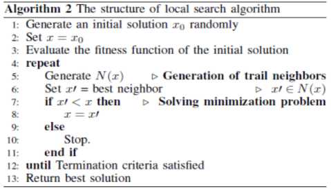
C. Local search algorithm

Local search algorithm (LSA) starts at a given initial solution. At each iteration, the heuristic replaces the current solution by a neighbor solution that improves the objective function. The search stops when all trail neighbors are worse than the current solution (local optimum is reached). Algorithm 2 illustrates the structure of a local search algorithm. In Algorithm 2, an initial solution x0 is generated randomly, from this solution a sequence of trail solutions x1, x2,..,xn are generated. If one of these trail solutions is better than the current solution, it becomes the current new solution. The operation is repeated until termination criteria satisfied.

D. Self-adaptive population resizing

GLSASAPR uses Algorithm 3 in order to reduce the population size and terminate the search automatically. The population is partitioning into υ partitions. The population vector PV is initialized to be 1 × k zero’s vector in which each entry of the i-th column in PV refers to a sub-population of NP as shown in Figure 1. While the search is processing, the entries of PV are not updated to be ones unless the fitness function value of the best chromosome in the current population size is ≤ Є, where Є = f best -f min /υ, υ, f best and f min represent the current population partitions number, best solution found in the current generation and the global optimum for the function. The entry of the last column in PV is updated to one when the fitness function value of the best solution in the population is equal or near the function global minimum value. At each time, the entry of the i-th column is updated to one and the population size is being reduced by 1/υ of the current population size during the evolutionary process by removing the worst chromosomes from the population. After having a PV full, i.e., with no zero entry, the search is learned that an advanced exploration process has been achieved and the algorithm is terminated.

E. The automatic termination criteria with PV

Termination criteria are the main GAs drawback. GAs may obtain an optimal or near-optimal solution in an early stage of the search but they are not learned enough to judge whether they can terminate. GLSASAPR uses the termination criterion of PV; the algorithm is terminated when all entries in PV are updated to be ones.

Algorithm 3 Self-adaptive population resizing

I: Partition P into v partitions
2: Assign each partition in P to its conesponding column in PV
3: Evaluate the fitness function of all individuals in P
4: if /best < e and NP > к then
5: Remove NPJv worst individuals from P
6: Update NP.
7: Choose i-th zero position in PV and update it to I
8: Set V = V - 1
9: else

to: if NP < к and Jbeet < ti then

11: Select the best individual from P
12: Update the last column in PV to I
13: end if
14: end if

F. The algorithm of GLSASAPR

The main steps of GLSASAPR algorithm is described as follows. GLSASAPR starts by setting the initial values of the population size NP, the crossover and mutation probabilities and the population vector PV. Then the initial population contains NP chromosomes (individuals) is created. At generation t, each individual in GLSASAPR is evaluated and the parent selection is applied. In order to generate a new offspring, GLSASAPR apply a linear crossover operator as shown in Procedure 1 and mutation operator. The population individuals are evaluated and the best found solution is refined by applying local search algorithm as an intensification process as shown in Algorithm 2. The population size reduction mechanism starts by applying Algorithm 3. This scenario is repeated until the termination criteria are satisfied. Specifically, GLSASAPR terminate the search after getting a full PV i.e with all ones.

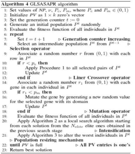
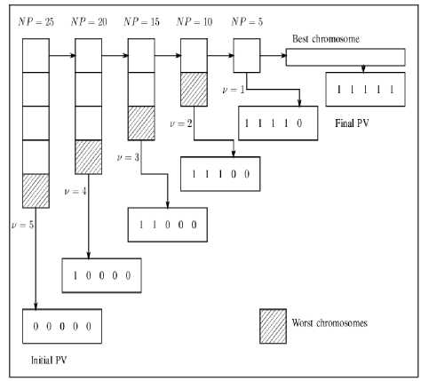
Fig 1: Population resizing mechanism

the initial population partitions.

The initial population of candidate solutions was generated randomly across the search space. The experimental studies show that, the best initial value of population size is NP = 25. The increasing of this value will increase the function evaluation value without much improving in the function values. The population size is decreased during the evolutionary process. The population size is divided to υ partitions, where υ = 5,...,1. The population size reduction is calculated as follows.

jy p (n w)

■I

N P ^)l^ -------; if p ^0) = 1

NP ^{(01 d)} ; if P V^(j ) = 0

IV. Numerical Experiments

In our experiments, fifteen benchmark classical functions f1 - f15 with different properties have been used to test the performance of GLSASAPR. The fifteen benchmark classical functions are reported in Table 5 in Appendix A. GLSASAPR was programmed in MATLAB, the results are reported in Tables 2, 3. Before discussing the results, we discuss the parameters setting of GLSASAPR algorithm and its performance analysis.

A. Parameter setting

GLSASAPR parameters are summarized with their assigned values in Table 1. These values are based on the common setting in the literature of determined through our preliminary numerical experiments. The parameters are categorized in the following groups.

Table1: Parameter settings

Parameters	Definitions	Values
NP	Initial population size	25
υ	Initial number of population partitions	5
k	Number of population vector columns	5
P c	Probability of crossover	0.6
P m	Probability of mutation	0.04
N elite	No. of best solutions for intensification	1

Population vector parameters (PV)

The population vector is divided into k sub-range, where k = 5. This value is corresponding to the number of

Where j refers to each entry column in PV, j =1,..., k.

• Crossover and mutation parameters

The crossover probability Pc represents the proportion of parents on which a crossover operator will act. We set the value of Pc equal to 0.6. The mutation operator performs a random walk in the vicinity of a candidate solution. The experimental results show that it is better to set Pm equal to 0.04.

• Local search parameters

At each generation, we apply a local search algorithm as shown in Algorithm 2 starting from the N elite best solutions, we set N_elite = 1.

B. Performance analysis

1) The efficiency of the local search algorithm:

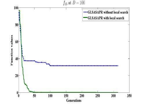
GLSASAPR uses a local search algorithm starting from the best obtained solution at each generation. The local search algorithm is invoked in GLSASAPR in order to accelerate the convergence at each generation instead of letting the algorithm running for several generations without much significant improvement of the objective function values. Figure 2 represents the general performance of GLSASAPR and the effect of the local search algorithm on two selected functions f11, f15 with 10, 30, 50, 100 dimensions by plotting the values of function values versus the number of generations.

In Figure 2, the dotted line represents the results of GLSASAPR without local search algorithm, the solid line represents the results of GLSASAPR with the local search algorithm. Figure 2 shows that the function values of GLSASAPR with applying the local search algorithm are decreases faster than the function values of GLSASAPR without local search algorithm as the number of function generation's increases.

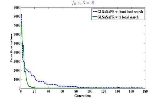
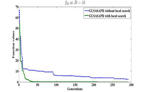
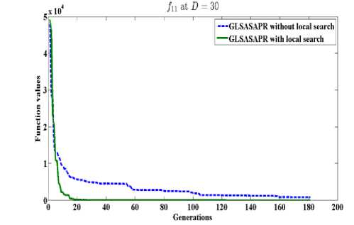
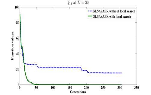
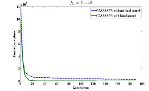
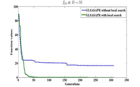
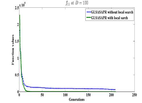
Fig. 2: The efficiency of applying the local search algorithm

2) The general performance of GLSASAPR on benchmark functions:

In order to analyze the general performance of GLSASAPR, numerical experiments on fifteen functions with 10 - 100 dimensions is studied as shown in Table 2 and Figure 3. The optimal solution results f(x*) are known for all benchmark functions. The benchmark functions and their properties are reported in Tables 5 in Appendix A. The mean of function evaluations (func-eval), function values (best func-val) and standard deviations for dimensions D = 10, 30, 50, 100 are reported in Tables 2. 30 runs were performed for each function. The results in Table 2 show that GLSASAPR found the exact global minimum value for 7 functions and near the optimal values for other 8 functions only with few thousands of function evaluations. Figure 3 also shows the general performance of GLSASAPR by plotting the values of objective functions versus the number of generations for functions f2, f3 at dimensions 10, 30, 50, 100. Figure 3 shows that the objective values are rapidly decreases as the number of function generations increases.

C. GLSASAPR and other Algorithms

GLSASAPR algorithm has been compared with the following eight relevant genetic algorithms

• ALEP (Adaptive Levy Evolutionary programming) [22].

This algorithm uses evolutionary programming with adaptive Levy mutation in order to generate a new offspring.

• FEP (Fast Evolutionary programming) [23].

This algorithm uses evolutionary programming with Cauchy mutation to generate a new offspring for each generation.

• OGA/Q (Orthogonal Genetic Algorithm with Quantization) [24].

This algorithm uses an orthogonal design to construct crossover operator.

• M-L (Mean-value-Level-set) [25].

This algorithm tries to improve the mean of the objective function value on the level set.

• CGA-TS (Conventional Genetic Algorithm and Tabu Search).

This algorithm is a hybrid algorithm between Conventional GA and TS algorithm.

• HTGA(Hybrid Taguchi Genetic Algorithm) [26].

This algorithm is a hybrid algorithm that combining the Taguchi method and a genetic algorithm.

• LEA (Level-set Evolutionary Algorithm) [9].

This algorithm is a level set evolutionary algorithm for global optimization with Latin squares.

This algorithm combines a global search genetic algorithm in a course to fine resolution space with a local Tabu search algorithm

Table 2: Experimental results of GLSASAPR for f1(x) - f15(x) with dimension D = 10, 30, 50, 100.

Function	D	Mean(func-eval)	Mean(best func-val)	Std.dev
f 1 (x)	10	1215.3	-12569.5	0.00
	30	1326.2	-12569.5	0.00
	50	1415.3	-12569.49	5.4E-04
	100	1826.4	-12569.35	5.7E-01
f 2 (x)	10	1189.5	0.00	0.00
	30	1328.67	0.00	0.00
	50	1426.83	0.00	0.00
	100	1534.5	0.00	0.00
f 3 (x)	10	1483.83	0.00	0.00
	30	1662.5	0.00	0.00
	50	1742	0.00	0.00
	100	1784.83	0.00	0.00
f 4 (x)	10	1162.17	0.00	0.00
	30	1286	0.00	0.00
	50	1291.5	0.00	0.00
	100	1351.33	0.00	0.00
f 5 (x)	10	1945.5	1.25E-07	1.11E-07
	30	2123.4	1.15E-07	9.14E07
	50	2133.5	2.31E-07	2.11E-07
	100	2185.7	2.46E-07	1.45E-07
f 6 (x)	10	2314.14	5.14E-06	2.24E-05
	30	2415.26	3.26E-06	5.12E-6
	50	2512.14	4.78E-06	3.12E-06
	100	2738.19	3.26E-06	2.14E-05
f 7 (x)	10	2931.4	-96.23	5.48E-06
	30	3894.6	-95.89	6.14E-06
	50	3965.4	-95.65	5.48E-05
	100	4285.4	-93.89	5.36E-05
f 8 (x)	10	1712.3	6.58E-08	5.89E-07
	30	1815.2	4.21E-08	6.32E-07
	50	1928.14	9.24E-07	2.48E-06
	100	2345.89	8.46E-07	4.58E-06
f 9 (x)	10	1524.8	-78.33	0.00
	30	1615.4	-78.33	0.00
	50	1756.2	-78.32	2.47E-04
	100	2110.3	-78.31	6.58E-03
f 10 (x)	10	1634.5	4.64E-01	2.14E-01
	30	4686.83	3.78E-01	6.4E-01
	50	7706.83	4.03E-01	2.58E-01
	100	15,243.17	4.71E-01	1.17E-01
f 11 (x)	10	923	0.00	0.00
	30	1083.83	0.00	0.00
	50	1135.67	0.00	0.00
	100	1201.67	0.00	0.00
f 12 (x)	10	2152.67	3.38E-03	3.31E-03
	30	4785.67	2.91E-03	2.10E-03
	50	7795.67	2.33E-03	2.66E-03
	100	15,333	1.39E-03	1.03E-03
f 13 (x)	10	1078.17	0.00	0.00
	30	1256.17	0.00	0.00
	50	1272.67	0.00	0.00
	100	1322.67	0.00	0.00
f 14 (x)	10	1330.84	0.00	0.00
	30	1606.16	0.00	0.00
	50	1741.17	0.00	0.00
	100	1913.67	0.00	0.00
f 15 (x)	10	1826.83	0.00	0.00
	30	2067.67	0.00	0.00
	50	2144.83	0.00	0.00
	100	2225	0.00	0.00

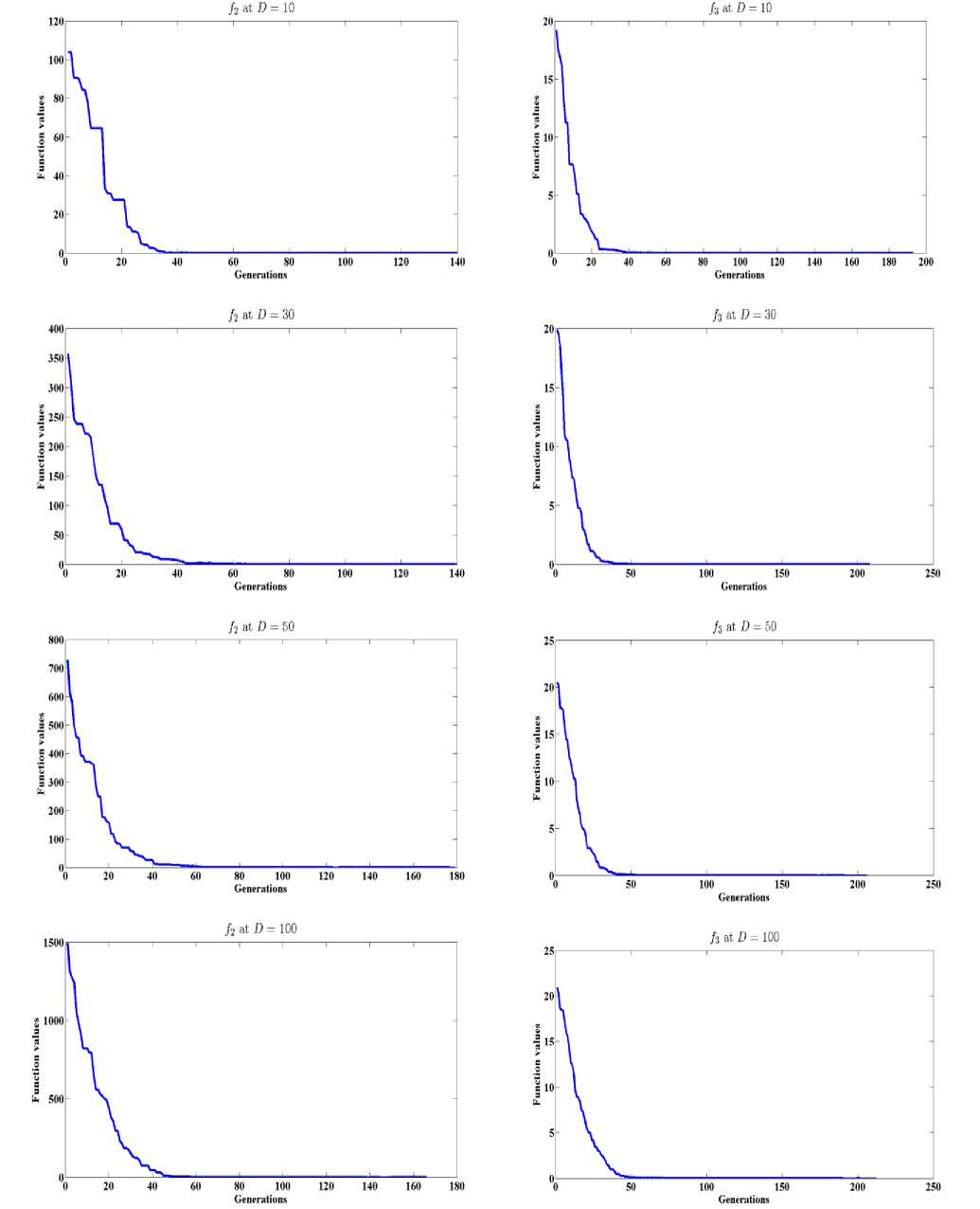
Fig. 3: The general performance of GLSASAPR

1) Comparison between GLSASAPR and other

algorithms

This section shows the comparison between

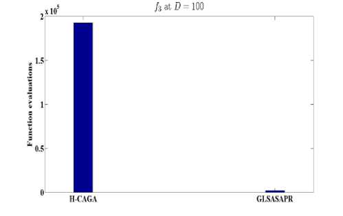
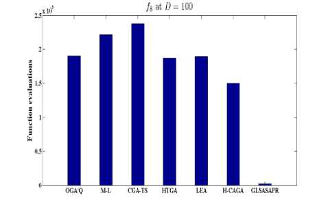
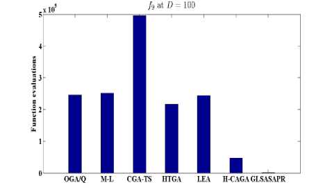
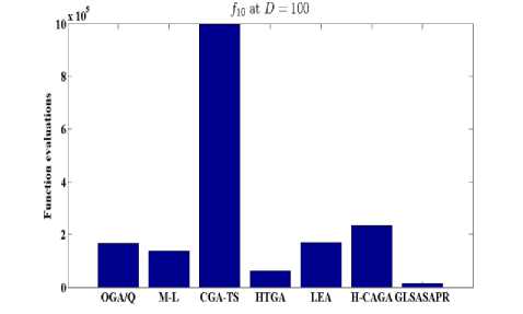
GLSASAPR and eight relevant genetic algorithms as described in the previous section. All algorithms are tested on fifteen benchmark functions f1-f15 as defined in Table 5 in Appendix A. The mean of function values, function evaluations and the standard deviation at dimensions 30 and 100 for eleven and four functions respectively are reported in Table 3 and Tables 4. The numerical results of all methods are taken from its original papers. We can conclude from the results in Table 3 and Tables 4 that GLSASAPR algorithm founded global optimum or near global minimum in many cases with low computational cost and outperformed the other algorithms. Also we can observed from Figures 4 and 5 that in the case of GLSASAPR, the error is close to 0 in most functions. Figures 4 and 5 show the mean error (using log values for a better visualization when the values are too low) for 30 and 100 dimensions for eleven and four functions respectively. For most of the other algorithms there could be observed an increase in error as the dimensionality of the problem increases. Figures 6 and 7 show the comparative results of GLSASAPR (function evaluations) and other algorithms at dimensions 30, 100 respectively. In Figures 6 and 7 the comparisons with other algorithms indicate that GLSASAPR is promising and it is less expensive and much cheaper than other algorithms

V. Conclusion

This paper presents a new hybrid algorithm for solving the nonlinear unconstrained global optimization problems. The proposed algorithm combines the GA and the local search algorithm in order to increase the ability of the diversification and the intensification of the algorithm. The proposed algorithm is called a Genetic Local Search Algorithm with Self-Adaptive Population Resizing (GLSASAPR). GLSASAPR invokes two main strategies. The first one is the population size reduction which reduces the cost of the evaluation function during the search process. The second strategy is the intensification process, which applies a local search algorithm at each generation in order to improve the best individual found so far. Moreover, a new termination criterion has been proposed by applying the population vector PV which is a zero’s vector in order to reduce the population size during the evolutionary process and terminates the search when all the zero entities of PV column updated to one’s. GLSASAPR has been compared with eight relevant genetic algorithm on fifteen benchmark test functions. The experimental results show that GLSASAPR is an efficient and promising algorithm and faster than other algorithms.

Table 3: Comparative results of GLSASAPR with other genetic algorithms for f1(x) - f8(x)

f	Algorithm	Mean (func-eval)	Mean (best func-val)	Std.dev
f 1 (x)	ALEP	150,000	-11469.2	58.2
	FEP	900,000	-12554.5	52.6
	OGA/Q	302,116	-12569.45	6.4E-04
	M-L	655,895	-5461.826	275.15
	CGA-TS	245,500	-12561.7	7.8
	HTGA	163,468	-12569.46	0.00
	LEA	287,365	-12569.45	4.8E-04
	H-CAGA	53,050	-12569.39	9.0E-01
	GLSASAP R	1326.2	-12569.5	0.00

f 2 (x)	ALEP	150,000	5.85	2.07
	FEP	500,000	0.046	0.012
	OGA/Q	224,710	0.00	0.00
	M-L	305,899	121.75	7.75
	CGA-TS	98,900	13.78	13.53
	HTGA	16,267	0.00	0.00
	LEA	223,803	2.1E-18	3.3E-18
	H-CAGA	15,658	0.00	0.00
	GLSASAP R	1328.67	0.00	0.00
f 3 (x)	ALEP	150,000	0.019	0.0010
	FEP	150,000	0.018	0.021
	OGA/Q	112,421	4.4E-16	3.9E-17
	M-L	121,435	2.59	0.094
	CGA-TS	242,700	0.00	0.00
	HTGA	16,632	0.00	0.00
	LEA	105,926	3.2E-16	3.0E-17
	H-CAGA	18,900	0.00	0.00
	GLSASAP R	1662.5	0.00	0.00
f 4 (x)	ALEP	150,000	0.024	0.028
	FEP	200,000	0.016	0.022
	OGA/Q	134,000	0.00	0.00
	M-L	151,281	0.1189	0.0104
	CGA-TS	245,600	4.7E-04	7E-04
	HTGA	20,999	0.00	0.00
	LEA	130,498	6.1E-16	2.5E-17
	H-CAGA	27,825	0.00	0.00
	GLSASAP R	1286	0.00	0.00
f 5 (x)	ALEP	150,000	6.0E-06	1.0E-06
	FEP	150,000	9.2E-06	3.6E-06
	OGA/Q	134,556	6.0E-06	1.1E-06
	M-L	146,209	0.21	0.036
	CGA-TS	440,500	1.85	1.857
	HTGA	66,457	1.0E-06	0.00
	LEA	132,642	2.4E-06	2.3E06
	H-CAGA	65,450	1.0E-06	9.9E12
	GLSASAP R	2185.7	2.46E-07	1.45E-07
f 6 (x)	ALEP	150,000	9.8E-05	1.2E-05
	FEP	150,000	1.6E-04	7.3E-05
	OGA/Q	134,143	1.9E-04	2.6E-06
	M-L	147,928	1.50	2.25
	CGA-TS	243,250	6.2E-06	0.00
	HTGA	59,033	1.0E-04	0.00
	LEA	130,213	1.7E-04	1.2E04
	H-CAGA	29,050	1.4E-06	2.1E-11
	GLSASAP R	2738.19	3.26E-06	2.14E-05
f 7 (x)	FEB	-	-	-
	OGA/Q	302,773	-92.83	0.03
	M-L	329,087	-23.97	0.62
	CGA-TS	496,650	-87.56	11.75
	HTGA	265,693	-92.83	0.00
	LEA	289,863	-93.01	0.02
	H-CAGA	244,600	-93.86	0.02
	GLSASAP R	4285.4	-93.89	5.36E-06
f 8 (x)	OGA/Q	190,031	4.7E-07	1.3E-07
	M-L	221,547	2.5E04	1.7E03
	CGA-TS	237,550	5.3E07	5.3E07
	HTGA	186,816	5.9E-05	8.3E-05
	LEA	189,427	1.6E-06	6.5E-07
	H-CAGA	150,350	5.2E-07	2.7E-12
	GLSASAP R	2345.89	8.46E-07	4.58E-06

Table 4: Comparative results of GLSASAPR with other genetic algorithms for f9(x) - f15(x)

f	Algorithm	Mean (func-eval)	Mean (best func-val)	Std.dev
f 9 (x)	ALEP	-	-	-
	FEP	-	-	-
	OGA/Q	245,903	-78.30	6.3E-03
	M-L	251,199	-35.80	0.89
	CGA-TS	495,850	-74.95	3.43
	HTGA	216,535	-78.30	0.00
	LEA	243,895	-78.31	6.1E-03
	H-CAGA	47,650	-78.19	0.53
	GLSASAPR	2110.3	-78.31	6.58E-03
f 10 (x	ALEP	-	-	-
	FEP	-	-	-
	OGA/Q	167,863	0.75	0.11
	M-L	137,100	2935.93	134.81
	CGA-TS	997,900	1072.80	1155.88
	HTGA	60,737	0.70	0.00
	LEA	168,910	0.56	0.11
	H-CAGA	234,250	1.4E-02	3.2E-03
	GLSASAPR	15,243.17	4.71E-01	1.17E-01
f 11 (x)	ALEP	150,000	6.3E-04	7.6E-05
	FEP	150,000	5.7E-04	1.3E-04
	OGA/Q	112,559	0.00	0.00
	M-L	162,010	3.19	0.29
	CGA-TS	146,900	3.6E-04	5.9E-04
	HTGA	20,844	0.00	0.00
	LEA	110,674	4.7E-16	6.2E-17
	H-CAGA	15,850	0.00	0.00
	GLSASAPR	1083.83	0.00	0.00
f 12 (x	ALEP	-	-	-
	FEP	-	-	-
	OGA/Q	112,652	6.3E-03	4.1E-04
	M-L	124,982	1.70	0.52
	CGA-TS	207,450	2.4E-03	2.5E-03
	HTGA	20,065	1.0E-03	0.00
	LEA	111,093	5.1E-03	4.4E-04
	H-CAGA	32,650	2.8E-06	1.5E-10
	GLSASAPR	4785.67	2.91E-03	2.10E-03
f 13 (x)	ALEP	-	-	-
	FEP	200,000	8.1E-03	7.7E-04
	OGA/Q	112,612	0.00	0.00
	M-L	120,176	9.74	0.46
	CGA-TS	146,900	3.6E-04	5.9E-04
	HTGA	14,285	0.00	0.00
	LEA	110,031	4.2E-19	4.2E-19
	H-CAGA	17,050	0.00	0.00
	GLSASAPR	1256.17	0.00	0.00
f 14 (x)	ALEP	150,000	0.04	0.06
	FEP	500,000	0.02	0.01
	OGA/Q	112,576	0.00	0.00
	M-L	155,783	2.21	0.504
	CGA-TS	145,500	7.8E-04	1.4E-03
	HTGA	26,469	0.00	0.00
	LEA	110,604	6.8E-18	5.4E-18
	H-CAGA	12,650	0.00	0.00
	GLSASAPR	1606	0.00	0.00
f 15 (x	FEB	500,000	0.3	0.5
	OGA/Q	112,893	0.00	0.00
	M-L	125,439	0.55	0.039
	CGA-TS	242,600	0.79	0.801
	HTGA	21,261	0.00	0.00
	LEA	111,105	2.6E-16	6.3E-17
	H-CAGA	725	0.00	0.00
	GLSASAPR	2067	0.00	0.00

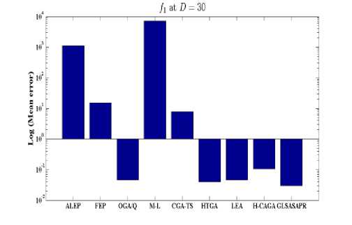
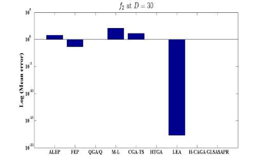
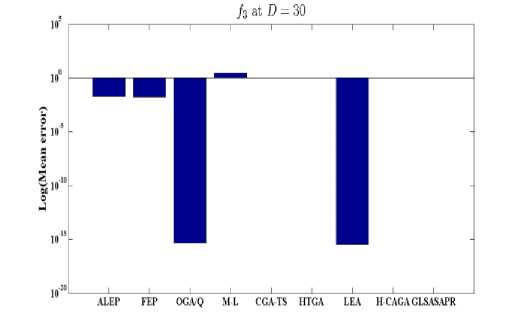
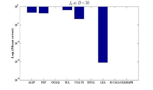
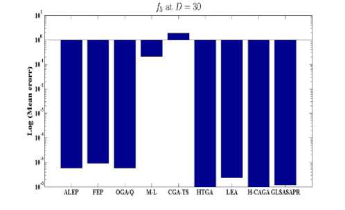
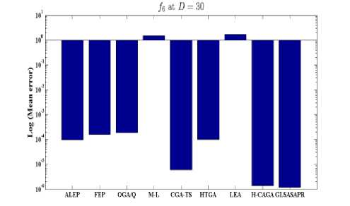
Fig. 4: Comparison of the increase in error between GLSASAPR and other algorithm at D = 30

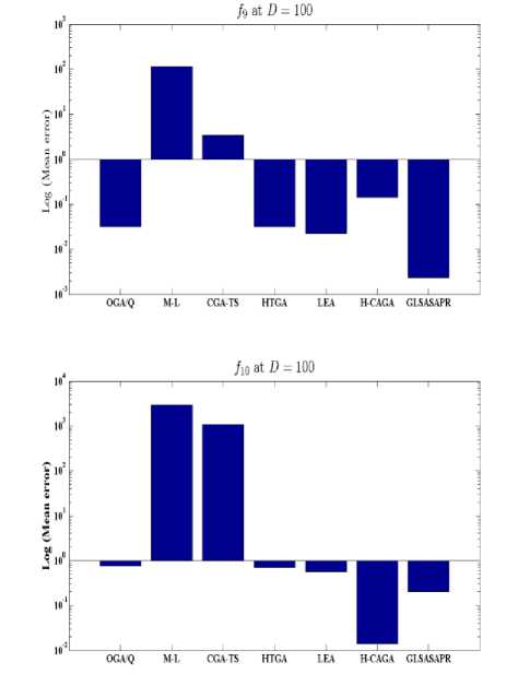
Fig. 5: Comparison of the increase in error between GLSASAPR and other algorithms at D = 100.

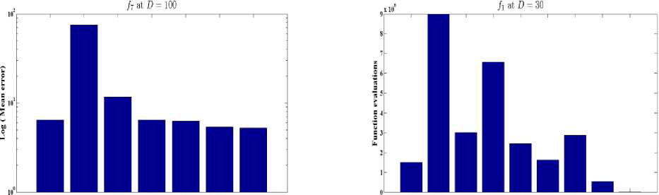
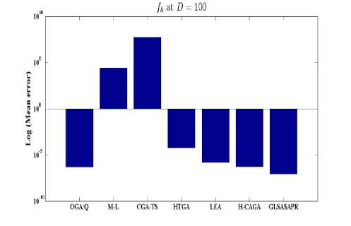
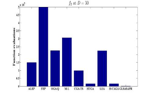
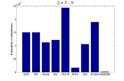
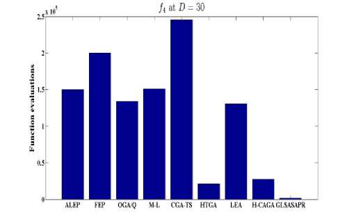
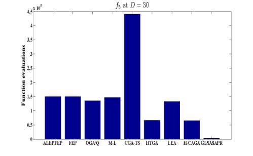
Fig. 6: Comparative results of GLSASAPR (function evaluations) and other algorithms at D = 30

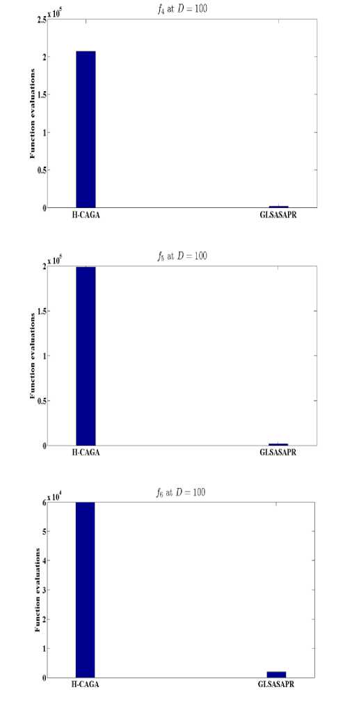
Fig. 7: Function evaluations of GLSASAPR and other algorithms at D=100

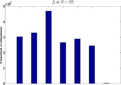
OGA/Q M-L CGATS HIGA LEA H-CAGA GLSASAPR

Appendix A:e Classical benchmark functions

Table 5: Classical benchmark function [27]

F	Fun_name	D	Bound	Optimum Value
F1	Schwefel’s problem 2.26	30	[-500,500]	-12569.5
F2	Rastrigin	30	[-5.12,5.12]	0
F3	Ackley	30	[-32,32]	0
F4	Griwank	30	[-600,600]	0
F5	Penalized levy1	30	[-50,50]	0
F6	Penalized Levy2	30	[-50,50]	0
F7	Michaelwicz	100	[0,π]	-99.2784
F8	-	100	[-π, π]	0
F9	-	100	[-5,5]	-78.33236
F10	Rosenbrock	100	[-5,10]	0
F11	Sphere	30	[-100,100]	0
F12	Quartic	30	[-1.28,1.28]	0
F13	Schwefel’s problem 2.22	30	[-100,100]	0
F14	Schwefel’s problem 1.2	30	[-100,100]	0
F15	Schwefel’s problem 2.21	30	[-100,100]	0

Список литературы Genetic Local Search Algorithm with Self-Adaptive Population Resizing for Solving Global Optimization Problems

C.T. Cheng, C.P. Ou, K.W. Chau, Combining a fuzzy optimal model with a genetic algorithm to solve multiobjectiverainfallrunoffmodelcalibration, Journal of Hydrology 268 (14) , 72-86, 2002.
F. Neri, V. Tirronen, Scale factor local search in differential evolution,MemeticComput. J. 1 (2) 153-171, 2009.
S. Kimura, A. Konagaya, High dimensional function optimization using a new genetic local search suitable for parallel computers, in: Proc. IEEE Int. Conf. Syst., Man, and Cybern., vol. 1, pp. 335-342, Oct. 2003.
N. Krasnogor, J.E. Smith, A tutorial for competent memetic algorithms: model, taxonomy, and design issue, IEEE Trans. Evol. Comput. 9 (5), 474-488, 2005.
D. Molina, M. Lozano, F. Herrera, Memetic algorithm with local search chaining for large scale continuous optimization problems, in: Proceedings of the 2009 IEEE Congress on Evolutionary Computation, Trondheim, Norway, pp. 830-837, 2009.
N. Noman, H. Iba, Accelerating differential evolution using an adaptive 948 local search, IEEE Transactions on Evolutionary Computation 12 (1)949 107-125, 2008.
V. Tirronen, F. Neri, T. Karkkainen, K. Majava, T. Rossi, An enhanced memetic differential evolution in filter design for defect detection in paper production, Evol. Comput. J. 16 (4), 529-555, 2008.
B. Liu, L. Wang, Y.H. Jin, An effective PSO-based memetic algorithm for flow shop scheduling, IEEE Trans. Syst. Man Cybern. 37 (1), 18-27, 2007.
Y. Wang, C. Dang, An evolutionary algorithm for global optimization based on level-set evolution and latin squares, IEEE Transactions on Evolutionary Computation 11 (5), 579-595, 2007.
W. Zhong, J. Liu, M. Xue, L. Jiao, A multiagent genetic algorithm for global numerical optimization, IEEE Transactions on Systems, Man, and Cybernetics-Part B, 34(2), 1128-1141, 2004.
H.K. Birru, K. Chellapilla, S.S. Rao, Local search operators in fast evolutionary programming, in: Proc. of the 1999 Congr. onEvol. Comput.,vol. 2, Jul., pp. 1506-1513, 1999.
J. H. Holland. Adaptation in Natural and Artificial Systems.University of Michigan Press, Ann Arbor, MI, 1975.
A.F. Ali, AE Hassanien, Minimizing molecular potential energy function using genetic Nelder-Mead algorithm, 8th International Conference on Computer Engineering & Systems (ICCES), pp. 177-183, 2013.
T. B¨ ack, D. B. Fogel, and T. Michalewicz. Evolutionary Computation:Basic Algorithms and Operators. Institute of Physics Publishing, 2000.
A. Hedar and A.F. Ali, and T. Hassan, Genetic algorithem and tabu search based methods for molecular 3D-structure prediction, International Journal of Numerical Algebra, Control and Optimization (NACO), 2011.
A. Hedar and A.F. Ali, and T. Hassan, Finding the 3D-structure of a molecule using genetic algorithm and tabu search methods, in: Proceeding of the 10th International Conference on Intelligent Systems Design and Applications (ISDA2010), Cairo, Egypt, 2010.
Z. Yang, K. Tang, X. Yao, Large scale evolutionary optimization using cooperativecoevolution, Information Sciences 178, 2985-2999, 2008.
A. Hedar, A.F. Ali. Tabu search with multi-levelneighborhood structures for high dimensional problems. Appl Intell, 37: 189-206, 2012.
M. Gong, L. Jiao, L. Zhang, Baldwinian learning in clonal selection algorithm for optimization, Information Sciences 180, 1218-1236, 2010.
P. Koro ˜ Sec, J. ˜ Silc, B. Filipic, The differential ant-stigmergy algorithm, Information Sciences 192 , pp. 82-97, 2012.
A. Wright, Genetic Algorithms for Real Parameter Optimization, Foundations of Genetic Algorithms 1, G.J.E Rawlin (Ed.) (Morgan Kaufmann San Mateo), 205-218, 1991.
C.Y. Lee, X. Yao, Evolutionary programming using mutations based on the levy probability distribution, IEEE Transactions on Evolutionary Computation 8 (1), 113, 2004.
X. Yao, Y. Liu, G. Lin, Evolutionary programming made faster, IEEE Transactions on Evolutionary Computation 3 (2), 82-102, 1999.
Y.W. Leung, Y.P. Wang, An orthogonal genetic algorithm with quantization for global numerical optimization, IEEE Transactions on Evolutionary Computation 5 (1) , 41-53, 2001.
C.S. Hong, Z. Quan, Integral Global Optimization: Theory, Implementation and Application, Springer-Verlag, Berlin, Germany, 1988.
J.-T. Tsai, T.-K. Liu, J.-H. Chou, Hybrid Taguchi-genetic algorithm for global numerical optimization, IEEE Transactions on Evolutionary Computation 8 365-377, 2004.
G. Garai, B.B. Chaudhurii, A novel hybrid genetic algorithm with Tabu search for optimizing multidimensional functions and point pattern recognition, Inform. Sci, 2012.

Еще

Статья научная

Genetic Local Search Algorithm with Self-Adaptive Population Resizing for Solving Global Optimization Problems

Текст научной статьи Genetic Local Search Algorithm with Self-Adaptive Population Resizing for Solving Global Optimization Problems

II. Global Optimization Problems

III. Genetic Local Search Algorithm With Self-Adaptive Population Resizing (Glsasapr)

• Population resizing

IV. Numerical Experiments

• Crossover and mutation parameters

• Local search parameters

V. Conclusion

Список литературы Genetic Local Search Algorithm with Self-Adaptive Population Resizing for Solving Global Optimization Problems