Getting Obstacle Avoidance Trajectory of Mobile Beacon for Localization

Published Online November 2010 in MECS

In many application areas of wireless sensor networks, such as object tracking, environment monitoring, health perception and ship navigation, the location information is critically essential and indispensable for it provides meaningful sensor data. Moreover, location information supports many fundamental network services including routing, topology and coverage control and so on [1].

The localization methods are classified into beaconbased or beacon-free. The beacon-based localization method needs some special sensor nodes (a.k.a. anchors or beacons or landmarks) know their global locations and the rest nodes (a.k.a. unknown nodes) determine locations by measuring the geographic information (e.g., distance or angle), which produces an absolute coordinate system. The beacon-free localization method is based on the network topology and produces a relative coordinate system. The former provides more precise position than the latter, but it is more expensive.

To decrease cost and keep accuracy of beacon-based localization methods, mobile beacon assisted localization algorithms are introduced and become promising. This method utilizes a mobile beacon to traverse the network deployment area to generate virtual beacons, and the unknown nodes estimate their locations with received virtual beacon positions. It is a basic and interesting problem in this method to obtain the optimal mobile beacon trajectory. The existing trajectory planning methods often suppose the network deployment area is obstacle-free, but there are many obstacles in real world, such as trees, rocks, holes. Therefore, this paper focuses on the planning of obstacle avoidance trajectory for mobile beacon.

The rest of the paper is organized as follows: Section II surveys various mobile beacon assisted localization and beacon trajectory-planning methods. Section III gives the obstacle-avoidance path planning method via fixed cell decomposition. Section IV describes the simulation and analyzes the results, and Section V concludes the paper.

• II.    Related Works

In beacon-based localization methods, the beacons are more expensive than unknown nodes. To reduce the number of static beacons, a mobile beacon is used to replace static beacons.

• A.    Mobile Beacon Assisted Localization Methods

The mobile beacon assisted localization methods can be classified as range - based and range - free , deterministic and probabilistic etc.

The range-based methods require the unknown nodes measure the distance to virtual beacons, and estimate their locations with trilateration or multilateration. Ref. [2] proposed a method using TDOA (Time Difference of

Arrival) of RF (Radio Frequency) and ultrasonic signal to range the distance and trilateration to estimate locations. MAL (Mobile Assisted Localization)[3] method employs a mobile user to assist in measuring distances between node pairs until these distance constraints form a “globally rigid” structure that guarantees a unique localization. The above are deterministic methods, and there are some probabilistic methods. Ref. [4] presented a method based on RSSI (Received Signal Strength Indicator) where the sensor nodes receiving beacon packets infer proximity constraints to the mobile beacon and use them to construct and maintain position estimates.

The range-free method estimates the unknown nodes with area or borderline measurement technology. The area measurement determines the area where unknown nodes located, and uses the centroid or weighted centroid as the location estimation. ADO (Arrival and Departure Overlap) algorithm [5] determines the arrival and departure area using a mobile beacon and estimates unknown nodes’ locations with centroid. Ref. [6] proposed a method based on geometric constraints utilizing three reference points. ADAL (Azimuthally Defined Area Localization) algorithm [7] uses a mobile beacon node equipped with a rotary directional antenna to determine the area.

The basic idea of borderline measurement is to determine two or more lines where an unknown node locates, and estimate its location as the cross point of these borderlines. Ref. [8] described a localization scheme using the conjecture of perpendicular bisector of a chord, which selects three virtual beacons to generate two perpendicular bisectors of chord and estimate locations. PI (Perpendicular Intersection) algorithm [9] is a similar method with different line-measurement method. The directional antenna and multi-power level mobile beacon can improve the localization accuracy [10, 11].

The probabilistic range-free schemes [12, 13] are based on SMC (Sequential Monte Carlo) method, which is composed of prediction and filter phases.

• B.    Mobile Beacon Trajectory Planning Methods

The traversal trajectory of the beacon in the deployment area is an interesting and basic problem to improve the localization performance. Ref. [4] presented some properties that the trajectory should have:

• (1)    The trajectory of the beacon should pass closely to as many potential node positions as possible for a node is best localized if the beacon is close to it.

• (2)    In two-dimension, the trajectory should ensure every node to be localized can receive at least three noncollinear beacon packets.

Furthermore, the trajectory should be as short as possible to be economic [14].

The trajectory planning schemes can be categorized into static and dynamic path planning method. The static method plans the mobile beacon trajectory before localization phase, and the beacon must follow the predefined trajectory during traversing the region. The RWP (Random Waypoint) model is usually used as the beacon trajectory [6, 12, 13]. In RWP model, the mobile beacon moves along a zigzag line from one waypoint to the next, and the waypoints are uniformly distributed over the given network deployment area. At the start of each leg, a random velocity is drawn from the velocity distribution (in the basic case the velocity is constant 1).

The RWP model cannot cover the entire network deployment region, which leads to some unknown nodes cannot be localized. In order to overcome this drawback, some deterministic trajectories are proposed. Three trajectories named by Scan, Double-Scan and Hilbert are studied in [15]. Scan is a simple and easily implemented trajectory composing of straight lines along one dimension, Double-Scan is to scan the network along both directions, and Hilbert is Hilbert filling curve. The simulation results showed that any deterministic trajectory that covers the whole area offer significant benefits compared to a random movement of the beacon. The localization algorithm with Hilbert as trajectory of beacon is investigated in [16], it defined the minimum Hilbert curve order that ensure the localization of all the unknown nodes, and claimed that the beacon must send its packets at every Hilbert key position.

Since straight lines invariably introduce collinearity, Ref. [17] designed Circles which consists of a sequence of concentric circles centered within the deployment area, and S-Curves which is based on Scan with ‘S’ curve instead of straight line.

To reduce beacon density and trajectory length, Ref. [18] proposed K-coverage trajectory that is designed to focus on the virtual beacon deployment and the shortest touring path obtainment, and a virtual force trajectory that is designed according to virtual force on mobile beacon that is exerted by unknown nodes. For the same reason, Ref. [14] deduced the number of virtual beacons according to the acreage of ROI (region of interest), and presented a method based on wandering sales representative problem algorithm to get the optimal path.

Regarding the wireless sensor network as a connected undirected graph, the path-planning problem is translated into having a spanning tree and traversing graph. Ref. [19] proposed breadth first and backtracking greedy algorithms for spanning tree to get the optimal trajectory.

The dynamic path planning methods try to give a realtime direction and step length of mobile beacon when it moves in the region. Ref. [20] provided a novel heuristic dynamic path planning method based on received-beacon numbers of ordinary nodes and deployed nodes in different regions using the directional antenna technology.

Besides the above trajectory planning method independent of localization algorithm, some localization schemes need special trajectory. For example, PI algorithm [9] requires the beacon to move in triangles.

All these methods supposed the deployment area is obstacle-free, they do not consider obstacle avoidance function when they planed the trajectory. However, there are many kinds of obstacles that the ground mobile beacon should avoid, thus this paper focuses on the obstacle avoidance trajectory-planning problem. The obstacle-avoidance routing protocol in sensor networks has been studied [21], which aimed at giving a shortest- path geographic routing in static sensor network using visibility-graph-based routing protocol.

III.    Obstacle Avoidance Path Planning

In robotics, the obstacle avoidance coverage path planning has been well-studied [22], and visibility graph and cell decomposition are two main methods. The main goals of path planning in robotics are to provide a shortest path cover a predefined area and avoid any obstacle along the path. For the trajectory planning of mobile beacon in wireless sensor network, the beacon need not cover all point of the deployment region while only need provide enough virtual beacons for each unknown node to localize [15].

• A.    Fixed Cell Decomposition

Cell decomposition is to partition a given region into disjoint sets, and let the robot travel the obstacle-free elements of the sets. Using the concepts in the field of robotics for reference, we introduce some terms and notions in first.

The deployment area of sensor network is configuration space C , and the obstacle-free part of C is denoted as C f_ree , the complement of C f_ree is C _obst . Each element of the disjoint sets after decomposition is called a cell , and a cell is called empty when it is in C free , and it is full when it is in C obst , and otherwise it is mixed . Cell decomposition method can be classified as exact and approximate . The idea of exact cell decomposition is to decompose C free into a collection of non-overlapping cells such that the union of all the empty cells exactly equals C f_ree . On the contrary, approximate cell decomposition is to construct a collection of non-overlapping cells such that the union of all the empty cells approximately covers C free . If all cells have equal size, it is fixed cell decomposition; otherwise, it is adaptive cell decomposition. After decomposition, C free can be mapped into connectivity graph G that is an undirected graph whose vertices correspond to empty cells and vertices connected by edge if and only if corresponding cells are adjacent. Note that, for a cell, not only the cells sharing common edges with it are adjacent cells (Fig.1(a)), but the four diagonal cells are adjacent as Fig.1(b).

This paper studies the obstacle avoidance trajectory planning with fixed cell decomposition, and the other methods will be discussed in future. For simplicity, we assume that:

• (1)    The mobile beacon can be modeled as a point, thus

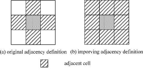
Figure 1. Adjacency definition.

the beacon can move freely in any size of empty cell.

• (2)    All the full and mixed cells will not be contained in the trajectory.

• (3)    C free is a continuous region, i.e., there is not any obstacle partitioning C into two disjoint parts. Consequently, the corresponding connected graph G is really connected (any pair of vertices of G have a path). This assumption implies that all the obstacles are solid.

• (4)    The cell decomposition uses square as cell shape.

The trajectory among empty cells is named by global trajectory , and that within each empty cell is local trajectory . The trajectory consists of global and local trajectory is called complete trajectory .

• B.    Global Trajectory Planning with Depth First Search

Since the deployment area is modeled by a connectivity graph G after cell decomposition, the global trajectory-planning problem is to present a shortest path traversing all vertices of G . We can use depth-first search to solve this problem. Suppose G =( V , E ) where V ={ v i | i =1,2,…, n } and E ={ e j | j =1,2,…, m }, algorithm 1 describes this method.

Algorithm 1 : GLOBAL T RAJECTORY P LANNING WITH

Depth First Search

Input : connectivity graph G =( V , E )

Output : global trajectory P procedure DFS( G )

• 1:    for i=1 to n

• 2:    visit(i)=false; parent(i)=0;

• 3:    end for

• 4:    curr=1; visit(1)=true; vn=1; P = Φ ;

• 5:    while vn

• 6:     S ={v(j) |(v(curr),v(j)) ∈ E and visit(j)=false};

• 7:    if S ≠ Φ

• 8:     v(k)=any element of S ;

• 9:      P = P ∪ {(v(curr),v(k)};

• 10:    parent(k)=curr;

• 11:    vn=vn+1;

• 12:     visit(k)=true;

• 13:     curr=k;

• 14:    else

• 15:     P = P ∪ {v(curr),v(parent(curr))};

• 16:    curr=parent(curr);

• 17:    end if

• 18:    end while

end procedure

Taking the number of adjacent cells into account, we adopt greedy strategy method to find an approximate shortest path. The basic idea of the greedy method is to make the path containing as less backtrack as possible. After visiting a vertex, the next vertex to visit is the one with the most adjacent and non-visited vertices. Algorithm 2 describes this method.

Algorithm 2 : GLOBAL T RAJECTORY P LANNING WITH

Greedy Strategy

Input : connectivity graph G =( V , E )

Output : global trajectory P procedure Greedy( G )

• 1:    for i=1 to n

• 2:    visit(i)=false;

• 3:    parent(i)=0;

• 4:    degree(i)=degree of v(i);

• 5:    end for

• 6:    degree(curr)=min{degree(i)|v(i) ∈ V };

• 7:    visit(curr)=true;

• 8:    vn=1; P = Φ ;

• 9:    for i=1 to n

• 10:    if (v(i),v(curr)) ∈ E

• 11:    degree(i)=degree(i)-1;

• 12:    end if

• 13:    end for

• 14:    while vn

• 15:    S ={v(j)|(v(curr),v(j)) ∈ E and visit(j)=false};

• 16:    if S ≠ Φ

• 17:    degree(k)=min{degree(i)|v(i) ∈ S };

• 18:     P = P ∪ {(v(curr),v(k)};

• 19:     parent(k)=curr;

• 20:    vn=vn+1;

• 21:     visit(k)=true;

• 22:     curr=k;

• 23:      for i=1 to n

• 24:         if (v(i),v(curr)) ∈ E and visit(i)=false

• 25:          degree(i)=degree(i)-1;

• 26:        end if

• 27:      end for

• 28:    else

• 29:        P = P ∪ {v(curr),v(parent(curr))};

• 30:       curr=parent(curr);

• 31:    end if

• 32:    end while

end procedure

The vertex with minimal degree is the vertex to visit firstly (line 6,7), and the degree of vertices adjacent to current visiting vertex is decreased by 1(line 9-13, 23-27). If the current visiting vertex v ( curr ) has no non-visited neighbors, the algorithm backtracks to its parent vertex (line 29-30); otherwise, selects the non-visited neighbor with minimal degree to visit (line17-22).

• C.    Global Trajectory Planning with AC Algorithm

The goal of global trajectory is to give the shortest path traversing each vertex, so we can regard it as TSP (Traveling Salesman Problem), which is a NP-hard problem. Ant colony (AC) algorithm can solve TSP well [23], so we can use ant colony algorithm to plan the global trajectory. However, the connectivity graph G may not have Hamilton cycle, so the shortest global trajectory may contain backtracks. Algorithm 3 presents this method, which is an ant-cycle algorithm with m = n ants. Algorithm 3 : G LOBAL T RAJECTORY P LANNING WITH A NT

Colony Algorithm

Input : connectivity graph G =( V , E ), maximum number of iteration iter_max and parameters α, β, ρ, Q

Output: global trajectory P procedure ACA(G,α,β,ρ,Q,iter_max,)

• 1:    for i=1 to n

• 2:    tabu(i,1)=i;

• 3:    for j=1 to n

• 4:       dis(i,j)=distance between v(i) and v(j);

• 5:        η(i,j)=1/dis(i,j); τ(i,j)=1;

• 6:       visit(i,j)=false; Δ τ(i,j)=1;

• 7:    end for

• 8:    visit(i,i)=true;

• 9:    end for

• 10:    while iter<=iter_max

• 11:    for i=2 to n//for the other n-1 vertices

• 12:       for j=1 to n// for all the ants

• 13:         r=i-1; u=tabu(j,r); tp=0;

• 14:         S ={k|visit(j,k)=false and dis(u,k)< ∞ };

• 15:         while length( S )==0

• 16:             r=r-1; u=tabu(j,r);

• 17:             S ={k|visit(j,k)=false and dis(u,k)< ∞ };

• 18:         end while

• 19:          for k=1 to length( S )

• 20:            p(k)= η(u,S(k))^βτ(u,S(k))^α;

• 21:            tp=tp+p(k);

• 22:         end for

• 23:          for k=1 to length( S )

• 24:            p(k)=p(k)/tp;

• 25:         end for

• 26:        p(v)=max{p(k)|S(k) ∈ S };

• 27:         tabu(j,i)=S(v);

• 28:      end for

• 29:    end for

• 30:    for i=1 to n

• 31:     len(i)=0;

• 32:     for j=1 to n-1

• 33:        if dis(tabu(i,j),tabu(i,j+1))< ∞

• 34:         len(i)=len(i)+dis(tabu(i,j),tabu(i,j+1));

• 35:        else

• 36:           for k=j-1 to 1 step -1

• 37:             if dis(tabu(i,k),tabu(i,j+1)) < ∞

• 38:              len(i)=len(i)+dis(tabu(i,k),tabu(i,k+1));

• 39:             else

• 40:              break;

• 41:             end if

• 42:          end for

• 43:       end if

• 44:       len(i)=len(i)+dis(tabu(i,j),tabu(i,j+1));

• 45:    end for

• 46:    end for

• 47:    k=min{len(i)|i=1,2,…,n};

• 48:    for j=2 to n

• 49:      if dis(tabu(k,j),tabu(k,j-1))< ∞

• 50:         P = P ∪ {tabu(k,j),tabu(k,j-1)};

• 51:      else

• 52:          for i=j-1 to 1 step -1

• 53:             if dis(tabu(k,j),tabu(k,i))< ∞

• 54:               break ;

• 55:             else

• 56:                P = P ∪ {tabu(k,j),tabu(k,j-1)};

• 57:         end for

• 58:         P = P ∪ {tabu(k,j),tabu(k,i)};

• 59:      end if

• 60:    end for

• 61:    for i=1 to n

• 62:       for j=1 to n-1

• 63:        u= tabu(i,j); v= tabu(i,j+1);

• 64:         Δ τ(u,v)= Δ τ(u,v)+Q/len(i);

• 65:      end for

• 66:    end for

• 67:    for i=1 to n

• 68:      for j=1 to n

• 69:        T^(i,j)=pT^{(i,j)+ А} т(ц);

• 70:        tabu(i,j)=0;

• 71:      end for

• 72:    end for

• 73:    iter=iter+1;

• 74:    end while

end procedure

Initially, the ant k ( k =1,2,…, n ) is on the vertex v ( k ) (line 2). Then, ant k selects the next vertex to visit according to the pheromone amount on the corresponding edge and transition probability p of each vertex (line 1327). After all ants visiting the entire graph (line 11-29), the length of each traversing path is computed (line 3046). Then, the shortest path is chosen (line 47-60) to update the global pheromone amount (line 61-72). The approximate shortest path is obtained after iter_max iterations (line 10-74).

• D.    Complete Trajectory Planning

The local trajectory can utilize any existing path, such as Scan, Hilbert, etc. Combining the global and local trajectory, algorithm 4 presents the complete trajectory planning method. Because the global trajectory excludes mixed and full cells, the complete trajectory can avoid obstacles.

Algorithm 4 : C OMPLETE T RAJECTORY P LANNING Input : configuration space C

Output : obstacle avoidance trajectory procedure CTP( C )

• 1:    Decomposing C with fixed cell decomposition

• 2:    Mapping C free to G

• 3:    Obtaining global trajectory by algorithm 1/2/3

• 4:    repeat

• 5:    Localizing the nodes in current empty cell

• 6:    Moving to next cell along the global trajectory

• 7:    while this empty cell is localized

• 8:       Moving to its parent cell on the global trajectory

• 9:    end while

• 10:    until all the empty cells are localized

end procedure

IV. Performance Evaluation

• A.    Simulation Setup

We use Matlab 7.0 to simulate above algorithms. Since localization precision results from the localization method and local trajectory, we only focus on analyzing the trajectory length and number of localizable sensor nodes. For simplicity, we assume that:

• (1)    The configuration space C is a square. If it is not a square, we can expand it by a circum-square to represent the area approximately. The cell shape can be square.

• (2)    The obstacles are all solid polygons, then each obstacle can be denoted by a series of vertices ( x i , y i ),

where x i , y i are the X- and Y-coordinate of i th vertex of a obstacle respectively.

• (3)    All the unknown nodes can be localized located in any empty cell.

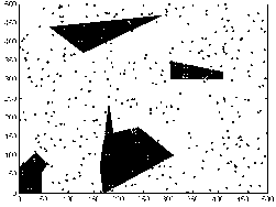
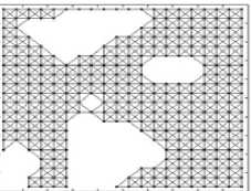
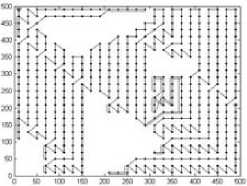
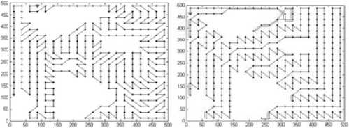
The configuration space C as the experimental environment is Fig.2(a), which is a 500*500m² space with 300 sensor nodes, and 33 nodes are in C obst (white hollow dots) while others are in C free (black solid dots). The black polygons are obstacles. The cell size is 50*50m², 25*25m², 20*20m² respectively. The parameters of ant colony algorithm are α=0.5, β=1, ρ=0.9, Q=2, iter_max= 20.

• B.    Simulation Results and Analysis

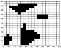
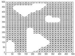
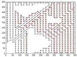
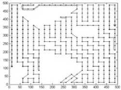
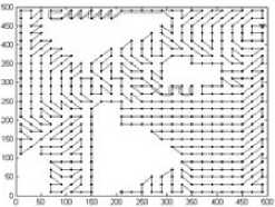
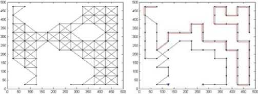
As an example, Fig.2(b) illustrates the decomposition result with cell 25*25m², where the white cells are empty and black cells are mixed or full. The connectivity graph G and corresponding global trajectories obtained by algorithm 1-3 are Fig. 3-5 respectively. The ‘*’ denotes the vertex to be visited first, and ‘ ∆ ’ denotes the vertex to be visited at the end. The black dots are vertices. The double lines of global trajectories are backtracks.

• (1)    Localizable unknown nodes in one-hop range. The number of localizable unknown nodes in one-hop range reflects the coverage of the mobile beacon trajectory. Because the mobile beacon will not traverse the mixed and full cells, only the unknown nodes in empty cells can be localized.

The unknown nodes in C obst are useless nodes , for they cannot provide useful information; the others are useful nodes . Table 1 gives the numerical results. With the decrease of cell size, the number of empty cells and localizable unknown nodes increase rapidly.

There are 33 useless nodes in our simulation. When the cell size is 50*50m2, the complete trajectory can localize 74.5% useful nodes. If the cell is 20*20m2, some original mixed cells become empty, and 91% useful nodes are localizable.

• (2)    Trajectory length. The trajectory should be as short as possible to save energy of mobile beacon. If the connectivity graph G has a Hamilton path, its length is:

Len opti = ( n - 1 ) ^{l (1)} where n is the number of empty cells, and l is the distance between a pair of adjacent empty cells which equals the cell size. Len opti is also the lower bound of the global trajectory length.

If G has no a Hamilton path, the global trajectory must contain some backtracks. Therefore, its length is:

Leng lobail = ( n ^{- 1 +} m ) ^{1 (2)} where m is the number of backtracks.

are designed to compute the approximate optimal global path among empty cells. The simulation results indicate that smaller cell size leads to more localizable sensor nodes. Unfortunately, it also results in longer complete beacon trajectory. Therefore, how to make a balance between them is worthy of studying in the future works.

(a) configuration space (b) cell decomposition Figure 2. Configuration space for simulation and results of cell decomposition

(a) connectivity graph

(b) depth first search

(a) connectivity graph            (b) depth first search

(c) greedy search             (d) ant colony algorithm

Figure 3. Connectivity graph and global trajectory (20*20m2)

Suppose the local trajectory within an empty cell is Scan whose resolution (the distance between two successive parallel segments of the trajectory) is r , the length of local trajectory is:

(c) greedy search             (d) ant colony algorithm

Figure 4. Connectivity graph and global trajectory (25*25m2)

Len local

= nl

Therefore, the length of the complete trajectory is:

Len comp

3 n + m - 1 +   I 1

r J

And the lower bound of complete trajectory is: т ( П1 \

Len iower = 1 ³ n ^{- 1} + — 1 ¹

v r J

(a) connectivity graph            (b) depth first search

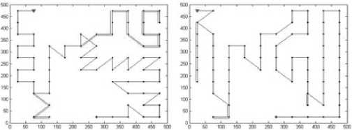
Table 2 gives the length of complete trajectory ( r =5m). If the cell is 50*50m², ant colony algorithm provides the shortest trajectory, but greedy strategy provides the shortest trajectory if the cell is 25*25m² and 20*20m². Moreover, the greedy strategy is faster than ant colony algorithm to obtain the global trajectory, so it is the best method among these three methods. Meanwhile, the complete trajectory becomes longer if the cell is smaller, regardless whatever the global trajectory is.

V. Conclusions and Future Works

The main contribution of this paper is to give a path planning method that can avoid obstacles. Using fixed cell decomposition, the sensor network deployment area are divided into many cells, and represented by a connectivity graph. Three algorithms including depth first search, greedy strategy method and ant colony algorithm

(c) greedy search             (d) ant colony algorithm

Figure 5. Connectivity graph and global trajectory (50*50m2)

Table 1. Number of each kind of cells and localizable nodes
Cell size(m)	Empty cells	Mixed cells	Full cells	Localizable nodes
50	69	30	1	199
25	314	69	17	232
20	500	92	33	243
Table 2. Length of complete trajectory (unit: m)
Cell size	DFS	Greedy	ACA	Lower bound
50	46750	45700	45200	44800
25	63275	62775	63325	62775
20	74680	70480	70820	69980

Acknowledgment

This work was supported in part by the National Natural Science Foundation of China under grants 60773034 and 60802030; The Natural Science Foundation of Shandong Province under grants ZR2009GQ002, ZR2010FQ014; Primitive Research Fund for Excellent Young and Middle-aged Scientists of Shandong Province under grant BS2009DX011.