GPU acceleration of edge detection algorithm based on local variance and integral image: application to air bubbles boundaries extraction

Bubbly flows are encountered in various industrial equipment such as, chemical reactions, purification of liquids, drag reduction of ships, gas/liquid contactors including bubble columns reactors, stirred tank reactors, evaporators, boilers and plate columns for absorption of gases and distillation. The knowledge of bubble characteristics is of crucial importance in determining the performance and in the study of various two-phase flow systems. The results of bubble dynamic are useful in extending the knowledge of bubble behavior in gas/liquid systems and in providing data to develop flow models. Bubble shape and dimensions play a key role in mass and heat transfer process between the dispersed and continuous phases.

Due to the action of hydrodynamic forces, the bubble shape would change. The interaction between rising bubbles and liquid determines the shape of the bubble and the extent of the disturbance in the surrounding fluid. Thus, instantaneous bubbles shapes, deformation of surfaces and sizes are very important because they reflect the dynamic changes of their pressures inside the bubbles and in the surrounding liquid. So, an improved understanding and instantaneous controlling of the flow around a rising gas bubble are required.

In recent years, digital image processing techniques have garnered research attention as a mean to analyze two-phase flow parameters, such as bubble deformation, gas fraction, rising velocity and flow velocity [1] and rising trajectory. Particularly, many studies to measure the bubble size have been performed involving the digital image processing techniques combined with high-speed imaging [2–7].

One of the fundamental and initial stages of digital image processing and computer vision applications is the edge detection. Examples of such applications include data compression, image segmentation, pattern recognition and 3D image reconstruction, etc. The success of the application depends on the quality of the resulted edge map, which is defined to consist of perfectly contiguous, well-localized, and one-pixel wide edge segments. The speed of edge detection technique is also of crucial importance especially for real-time applications. Particularly, accurate and rapid extraction of bubbles contours is an essential step for instant control of two-phase flow systems requiring an accurate estimation of air bubble parameters.

Today, the main challenge for developers in the field of image processing and computer vision is achieving high accuracy and real time performance. Most of image processing applications operate on higher resolution images, which requires intensive computation power and excessive computing time, especially if multiple tasks have to be performed on the image. In addition, in most cases, a common computation is performed on all pixels of the image. This structure matches very well GPU’s SIMD architecture (single instruction multiple data) and can be effectively parallelized and accelerated on the GPU.

Thus, many authors have exploited the programmable graphics processing units’ capabilities to improve the runtime of their algorithms. Numerous classic image processing algorithms have been implemented on GPU with CUDA in [8]. OpenVIDIA project [9] has implemented diverse computer vision algorithms running on graphics processing units, using Cg, OpenGL and CUDA. Furthermore, there are some works for GPU implementation of new volumetric rendering algorithms and magnetic resonance (MR) image reconstruction [10]. Moreover, several fundamental graph algorithms have been implemented on the GPU using CUDA in [11– 13].

Despite the fact that image processing algorithms match very well the massively parallel architecture of the GPU, a wide number of applications failed to achieve significant speedup due to architectural constraints and hardware limitations of the modern graphic cards that should be considered when the algorithm is ported to GPU.

The present study aims to develop an accurate edge detection algorithm performing in real-time, in order to extract edge map of air bubbles floating in static fluid in two-phase flow systems, for further processing later.

Due to the specificity of the bubble images, where the gray levels on the bubble boundary are not constant, which makes its extraction from the background accurately difficult, an edge detection algorithm based on local variance computation using integral image is improved and accelerated on the GPU in this study. The local variance-based method is robust against changes of intensity contrast between air bubbles and image background, and is able to provide strong and consistent edge responses on the boundaries of low contrast bubbles.

Our main contribution in this work is the efficient optimization techniques that have been introduced in our parallel implementation to reach real time execution. The proposed algorithm shows its efficiency when compared with those of state-of-the-art edge detection algorithms accelerated on the GPU.

The remainder of this paper is structured as follows: a review of the edge detection algorithms from the literature is introduced in Section 1. A description of the proposed algorithm is given in Section 2. Proposed in Section 3 is its GPU implementation. Experimental results obtained with the proposed algorithm and comparisons with those of state of the art are shown in Section 4. Finally, conclusions are given in the last Section.

1.    Review of edge detection algorithms

The edge detection task is a challenging problem, notably in case of blurred, low contrast and noisy image. Thus, it was broadly discussed over the years. Based on traditional techniques, many recent papers have exploited the gradient to detect image edges [14– 16]. Other approaches were inspired from the natural computing [1720], these techniques used neural network or membrane computing to detect edges. Type-2 fuzzy systems were also used to find image edges [16, 21], that can be combined with Sobel detector to reach the same purpose [21]. Also, numerous other methods based on different techniques have been developed, including the differentiation-based methods [22, 23], machine learning methods [24, 25], the anisotropic diffusion or selective smoothing methods [26], and multiscale methods [27, 28].

Furthermore, the author in [29] proposed an edge detector based on a local dimension of complex networks using the weighted combination of the Euclidean distance and gray-level similarity indices. More recently, the au- thor in [30] proposed an approach based on Faber Schauder Wavelet and Otsu threshold. In this algorithm, the image is firstly smoothed with a bilateral filter depending on noise estimation. Then, the Otsu’s method was applied to select the FSW extrema coefficients. Finally, the edge points are linked using a predictive linking algorithm to get the final edge map.

Nevertheless, the most of the existent edge detectors fail in producing confident results due to the noise, the non-uniform scene illumination and the image blur. The success of an edge detection algorithm depends on its capability to produce good localized edge maps with minimal effect of noise. Therefore, there is always a trade-off in the edge detection technique between extracting the information and suppressing the noise. Common edge detectors overcome noise by first smoothing images, typically with a Gaussian kernel. Such smoothing indeed reduces the noise, but may blur and weaken the contrast across edges, or even worse, blend adjacent edges.

Using diverse type of filters or transformations like morphological analysis [34], Hilbert transform [35], and multiple radon or beamlet transform [36] is not suitable to handle noise. Indeed, excessive use of these transformations and filters or the use of large scales could reduce their ability to detect short edges and create non-continuous edges.

Finally, edge detector based on machine learning [38, 39] is just making the problem more complicated and not practical. In addition, the performance is not guaranteed as this type of edge detection depends heavily on the training samples.

2.    Edge detection based on local variance

Generally, the measurement of bubbly flow parameters with digital image processing techniques starts by de- tecting edge of bubbles, and then uses edge map for further high-level processing. Most of these techniques use preprocessing approaches such as filtering to remove noise and thresholding to low-level feature extraction. Nevertheless, there are many limitations in the performance of these approaches. The performance of thresholding approaches is limited by the bubble size, noise, contrast, intensities difference between bubbles and the background, and variances of bubble and background. Minimizing noise by filtering operations results in blurred and distorted boundaries since both edges and noise contain high-frequency contents.

Due to these difficulties, preprocessing step must be applied in such a way as to not remove or distort the signal of interest, and the ideal solution is an approach that avoids the preprocessing step entirely.

The proposed algorithm is based on the exploitation of raw images in order to preserve all features details until the final phase of treatment. This edge detection technique is performed on two main steps: in the first step, the local variance of each pixel is computed based on integral image in order to improve computation time, and then the resulting contours are thinning to generate the final edge map. The principles of the two steps are described below.

• 2.1.    Variance calculation

The variance of the original image (in grayscale) is done on small window D centered on the pixel of coordinates ( x , y ) according to the following expression:

^2.,у) =Z (iv,j) -ц)2, (1) (i,j)eD where ц is the mean value of pixels intensities in the window D, and I(i,j) is the intensity of the pixel (x, y) to be processed in the input image.

The obtained result is the variance image representing the different contours of the detected patterns and preserving all the useful information.

According to Eq. 1, the local variance of a pixel is based on the average value computation of the window centered at this pixel. Thus, the number of summation operation, needed to the mean value calculation, will increase with the window size and consequently the execution time will increase. For every pixel in the input image, (4 ×w ²) arithmetic operations will be performed to generate the corresponding pixel variance value (where w is the size of the window along an axis). Consequently, the computational complexity of the variance computation of an image size of ( N × M ) pixels will be in the order of O (4× w ²× N × M ).

To eliminate this dependency and improve computation time, the integral image is used to compute the mean and variance of the processed image.

The variance of any region D of an image I using integral image approach can be calculated using the following formula:

^2x , у) = -1Ч D )-|-14D Л , (2) n V n / where I' and I'' are respectively, the integral image and the squared integral image of the input image I and n is the number of window D pixels.

• 2.2.    Contour thinning

3.    GPU implementation

• 3.1.    Integral_kernel

The contours generated by the first step have a certain thickness (greater than 1 pixel). Thus, a thinning phase is necessary to refine it. The local variance of a region across the edge of an image is bigger than those regions where no edge is crossed. Thus, the center pixel ( x , y ) of that region is an edge pixel. In this step, all the columns of the variance image are processed, in increasing and decreasing order, by eliminating all pixels having a smaller variance value than their successor or predecessor, respectively. The obtained result is a set of peaks corresponding to the detected local maxima. These peaks are the final contours of

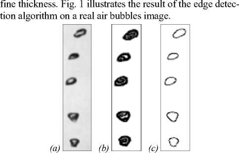
Fig. 1. Results of applying the edge detection method to real image of air bubbles: (a) original image, (b) transformed image and (c) contour image (the quality of contours may be deteriorated due to color inversion)

In the following, we detail the parallel implementation on the GPU of the edge detection algorithm. The algorithm is bifurcated into three principal steps: Integral and squared integral images computation, variance value calculation and contour thinning. In the integral image computation step, (5× N × M ) arithmetic operations are required for an image size of ( N × M pixels). Consequently, the computational complexity of this step will be in the order of O (5× N × M ). In the variance calculation step, for every pixel in the image 10 arithmetic operations will be performed to generate the corresponding pixel variance value. Thus, the computational complexity of this step will be in the order of O (10× N × M ). Finally, for the thinning step each pixel in the variance image performs 2 comparisons to generate the final fine contour. Hence, the total complexity of this step will be in the order of O (2× N × M ).

Therefore, the global time complexity of the algorithm will be in the order of O (17× N × M ). Since, our main goal is the acceleration of the computation time to reach real time, the three steps of the algorithm are transferred to the GPU, which we implemented three kernels, Integral_kernel, Var-iance_kernel and Thinning_kernel.

The value at any location (x, y) in the integral image is the sum of all the pixels intensities above and to the left of (x, y), inclusive. This can be expressed mathematically as follow:

I ( x , y ) =

I I (A y .

where I' and I are the values of the integral image and the input image respectively.

Equation (3) has potential for parallel computation, using the following recursive equations:

^S ( x , y ) = ¹ ( x , y ) + ^S ( x , y - 1) , I (x , y ) = I (x - 1, y ) + S ( x , y ) .

The first stage computes the cumulative row sum S at a position ( x , y ) in the image and forwards the sum to the second stage for computation of the integral image I' ( x , y ) value at that position.

This kernel is launched with a number of threads equal to the number of rows of the input image to be processed. These threads are arranged in one-dimensional thread blocks. Thus, the total number of thread blocks is the size of the input image divided by the number of threads. The computation of the integral image is performed in two steps: we assigned one thread to compute the cumulative sum of one row. Once all threads achieved calculation , each one of them performs the integral image value computation for the column assigned to it.

The following algorithm (1) illustrates the integral image computation: the input image is scanned, and for each row the cumulative sum is computed. Then, the integral image is calculated for each column. Finally, the results are stored in the global memory. Each thread computes its corresponding row index i , as:

i = (blockIdx.x + threadIdx.x × gridDim.x) × N , where gridDim.x is the number of blocks in the grid and N the width of the input image.

Algorithm 1: Integral_kernel

Input: the input image ( I ) and its height and width M , N Output: the Integral image ( I' )

• 1:    i ← (blockIdx.x + threadIdx.x × gridDim.x) × N ;

• 2:    for k ←0 to ( N –1) do // sweep the row pixels

• 3:    I ( i + k +1) ← I ( i + k ) + I ( i + k +1) ; // compute the cumulative sum for one row

• 4:    End;

• 5:    for k ←0 to ( M –1) do // sweep the column pixels

• 6:    I ( i +( k +1)× N ) ← I ( i + k × N ) + I ( i +( k +1)× N ) ; // compute the integral image for one column

• 7:    I' ( i +( k +1)× N ) ← I ( i +( k +1)× N ) ; // Store the integral image value in the global memory

• 8:    End;

• 3.2.    Variance_kernel

For this kernel, we mapped one thread to each pixel of the integral image returned by the Integral_kernel . (N×M) threads are generated to process (N×M) pixels. These threads are grouped in one-dimensional thread blocks. The following algorithm (2) illustrates the variance value computation: the integral and the squared integral images are scanned, and for each pixel the corre- sponding variance is computed. Then, the variance value is stored in the global memory. Each thread computes its corresponding pixel index i, as:

i = blockIdx.x + threadIdx.x × gridDim.x, where gridDim.x is the number of blocks in the grid.

Algorithm 2: Variance_kernel

Input: the integral image ( I' ), the squared integral image ( I'' ), N and w

Output: the variance image ( V )

• 1:    i ← blockIdx.x + threadIdx.x × gridDim.x;

• 2:    Fetch I' ( i +( w +1)+( w +1)× N ) , I' ( i – w – w × N ) , I' ( i +( w +1)– w × N )

and I' ( i – w +( w +1)× N ) from the global memory; // the 4 corners of the window in the integral image

• 3:    Fetch I'' ( i +( w +1)+( w +1)× N ) , I'' ( i – w – w × N ) , I'' ( i +( w +1)– w × N )

and I'' ( i – w +( w +1)× N ) from the global memory; // the 4 corners of the window in the squared integral image

• 4:    Compute v i using formula (3); // computing the variance value of the pixel i

• 5:    V i ← v i ; // Store the variance value in the global memory

• 3.3.    Thinning_kernel

The Thinning_kernel implementation takes a different approach from that of the Variance_kernel. A single thread processes an entire column of the variance image. Thus, the total number of threads in the grid corresponds to the number of columns ( N ) of the variance image ( V ). The threads sweep the columns in the ascending and in the decreasing order. Each thread compares the intensity of the tested pixel in the column assigned to it with that of its successor or predecessor according to the direction. If lower, it will be rejected. Else, it will be stored in the global memory as an edge pixel. The following algorithm (3) illustrates the Thinning_kernel procedure. Each thread computes its corresponding pixel index i , as:

i = (blockIdx.x + threadIdx.x × gridDim.x) × N .

Algorithm 3: Thinning_kernel

Input: the variance image ( V ), and its width N

Output: the edge image ( E )

• 1:    i ← (blockIdx.x + threadIdx.x × gridDim.x) × N ;

• 2:    for k ←0 to ( N –2) do // sweep the column in the ascending order

• 3:     if ( V ( i + k ) <  V ( i + k +1) ) // compare each pixel in the column

with its successor

• 4:           V ( i + k ) ←0;

• 5:    End;

• 6:    for k ←( N –1) to 1 do // sweep the column in the descending order

• 7:     if ( V ( i + k ) <  V ( i + k –1) ) // compare each pixel in the column

with its predecessor

• 8:           V ( i + k ) ←0;

• 9:      E ( i + k ) ← V ( i + k ) ; // Store the edge pixel value in the global

memory

• 10:    End;

We used CUDA streams to further optimize this kernel.

The Thinning_kernel can be divided into two tasks independent each from the other (sweeping the columns of the image in the ascending order firstly and in the decreasing order secondly).

Thus, we implemented two sub-kernels (Thin-ning_kernel_A and Thinning_kernel_D), one for each direction, with the same configuration of threads and blocs as the original implementation and we created two streams to launch these sub-kernels concurrently. A better performance is given by this asynchronous implementation compared to the basic one. The following algorithms (4 and 5) illustrate the two sub-kernels procedures.

Algorithm 4: Thinning_kernel_A

Input: the variance image ( V ), and its width N

Output: the edge image ( E )

• 1:    i ← (blockIdx.x + threadIdx.x × gridDim.x) × N ;

• 2:    for k ←0 to ( N –2) do // sweep the column in the ascending order

• 3:     if ( V ( i + k ) <  V ( i + k +1) ) // compare each pixel in the column

with its successor

• 4:        V ( i + k ) ←0;

• 9:    E ( i + k ) ← V ( i + k ) ; // Store the edge pixel value in the global memory

• 10:    End;

Algorithm 5: Thinning_kernel_B

Input: the variance image ( V ), and its width N

Output: the edge image ( E )

• 1:    i ← (blockIdx.x + threadIdx.x × gridDim.x) × N ;

• 2:    for k ← ( N –1) to 1 do // sweep the column in the descending order

• 3:     if ( V ( i + k ) <  V ( i + k –1) ) // compare each pixel in the column

with its predecessor

• 4:        V ( i + k ) ←0;

• 9:      E ( i + k ) ← V ( i + k ) ; // Store the edge pixel value in the global

memory

• 10:    End;

4.    Experimental results and analysis

• 4.1.    GPU implementation complexity analysis

• 4.2.    Optimization of execution configuration

  To achieve best performance, a serie of tests by varying the number of threads per block is carried out to determine the appropriate configuration that satisfies our real-time constraint, taking into account the resource usage of an individual thread. In this experiment, a set of tests on 300 images with different sizes ranging from (128×128) to (1024×1024) pixels, under several practical conditions was performed. For each test, 200 runs were carried out and the average execution time is reported for each kernel. Tables 2–4 illustrate the obtained results for each kernel.

The aim of these experiments is to confirm that with the capabilities of the programmable GPU, the speed of our algorithm will be considerably improved and reached real time execution. For this purpose, the computational performance of the GPU implementation with different sizes of images ranging from (128 × 128) to (1024 × 1024) pixels was compared to the CPU implementation. We used a computer equipped with an Intel® Core ™ i7-3770 CPU performing at 3.4 GHZ and 16 GB RAM. Also, it is equipped with an NVIDIA GeForce GTX 780 GPU. A detailed description of the used graphic card, in this work, is illustrated in Table 1. For the implementation of the algorithm we used the vs2015 configured with OpenCV 3.0.0, and the CUDA 6.5.

From Section 3, the overall computational complexity of the edge detection algorithm is in the order of O (17× N × M ) to process an image size of ( N × M ) pixels. In the Integral_kernel, N threads are launched to carry out computations, where each thread performs (2× M ) operations. Hence, the computational complexity of one thread is O (2× M ). The Variance_kernel is launched with ( N × M )

threads and each one performs 10 operations. Thus, the computational complexity of a single thread is O (10). The Thinning_kernel is launched with a total of ( N ) threads and each thread performs 2 operations. Hence, the computational complexity of each thread is O (2× M ).

Table 1. GPU hardware specification

Architecture	Kepler GK110
Compute capabilities	3.5
Base clock	863 MHZ
Cores CUDA	2304
Number of Streaming Multiprocessor	12
Maximum shared memory per SM	48KB
Maximum threads per SM	2048
Maximum blocks per SM	16
Maximum threads per block	1024

In practice, the execution time depends on the maximum number of threads that can be executed simultaneously by the GPU. In our case, a total of 2048 threads can be launched by each SM. Thus, a total of (2048×12) threads can be executed concurrently on the 12 SM of the GPU. Therefore, the total computational complexity of the edge detection algorithm is the sum of those of the three kernels divided by the total number of executed threads at a time, which is in the order of O ((10+6 × M ) /(2048 × 12)) and can be considered as O ( M /(2×2048)).

We can see that the best run time for the Inte-gral_kernel, the Variance_kernel and the Thinning_kernel is achieved when the number of threads is equal to 256, 512 et 32, respectively. This can be explained by the full use of blocks provided by the SM in these cases, which leads to maximize resources and consequently speed up execution time.

• 4.3.    Asynchronous execution assessment

In this section, we evaluate the effectiveness of the asynchronous implementation of the Thinning_kernel. Table 5 illustrates the execution times for the two implementations with different image sizes.

This Table shows that for all image sizes, the asynchronous implementation of the Thinning_kernel outperforms the basic implementation with a speedup factor approximately equal to 1.5×. For example, the run time for an image size of (1024×1024) pixels is decreased from 5.04 ms to 3.34 ms.

Table 2. Average execution times (µs) for the Integral_kernel

Image sizes (pixels)	32 threads	64 threads	128 threads	256 threads	512 threads	1024 threads
128×128	467.33	446.51	422.49	-	-	-
256×256	1033	937.14	889.07	884.66	-	-
512×512	2460	2070	1880	1860	2260	-
1024×1024	5960	4930	4170	3940	4710	7680
Table 3. Average execution times (µs) for the Variance_kernel
Image sizes (pixels)	32 threads	64 threads	128 threads	256 threads	512 threads	1024 threads
128×128	43.10	40.28	36.41	42.62	40.57	52.22
256×256	172.54	138.43	142.50	141.40	137.69	170.78
512×512	648.05	534.13	547	546.39	534.1	619.99
1024×1024	2520	2290	2170	2160	2100	2390
Table 4. Average execution times (µs) for the Thinning_kernel
Image sizes (pixels)	32 threads	64 threads	128 threads	256 threads	512 threads	1024 threads
128×128	378.23	379.69	380.68	-	-	-
256×256	802.45	809.17	809.04	856.27	-	-
512×512	1610	1620	1620	1700	2350	-
1024×1024	3340	3380	3345	3390	4690	8970

Table 5. Execution times (µs) for the two Thinning_kernel implementations with different image sizes

Image sizes (pixels)	Basic kernel	Asynchronous kernel
128×128	598	378
256×256	1280	802
512×512	2530	1610
1024×1024	5046	3340

4.4. Overall performance assessment

Table 6 illustrates the execution times and speedups for the CPU and GPU implementations of our edge detection algorithm for different image sizes. It is clear that the GPU approach outperforms the CPU implementation. We can see that considerable gains are achieved with the GPU implementation with respect to the serial implementation. For instance, a gain factor around 17× is reached with an image size of ( 1024x1024 ) pixels.

most commonly edge detection methods existing in the literature Sobel, Robert, Prewitt and Canny in terms of accuracy. Examples of results on 2 images are shown in Fig.2. From the qualitative results shown in this Figure, we can see that clear and continuous edges are successfully identified in all images with our algorithm. Despite the specificity of the bubble images, where the gray levels on the bubble boundary are not constant, which makes its extraction from the background difficult, a remarkably performance of our algorithm can be seen compared to the common methods which are failed to extract correctly the bubbles edges. Our algorithm can accurately extract edges even if images contain a non-uniform background and an obscure boundary.

Table 6. Execution times (msec) on CPU and GPU of the edge detection algorithm and speedup factors

4.5. Comparison with state of the art

In addition, to further prove the effectiveness of the proposed algorithm, we compared it with those of state-

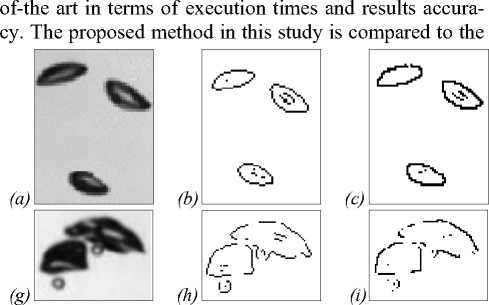
Fig. 2. Edge detection results comparison with state of the art: (a, g) original images, (b, h) Sobel, (c, i) Robert, (d, j) Prewitt, (e, k) Canny and (f, l) our algorithm (the quality of contours may be deteriorated due to color inversion)

Image sizes (pixels)	CPU	GPU	Speedup
128×128	104	1.259	82.6
256×256	130	2.763	47.05
512×512	153	5.864	26.09
1024×1024	233	13.320	17.49

(l)

(f)

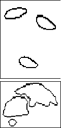
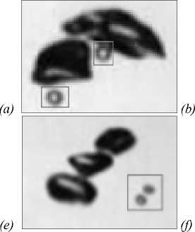
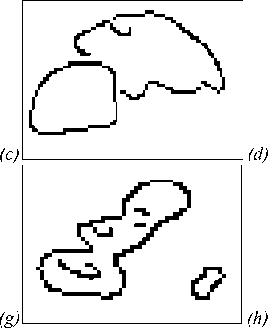
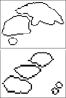
Fig. 3. Edge detection results: comparison of our algorithm with Canny operator: (a, e) original images, (b, f) Canny; Tresh = 0.3, (c, g) Canny; Tresh = 0.7 and (d, h) our algorithm (the quality of contours may be deteriorated due to color inversion)

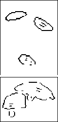
In a second test we compared the performance of our algorithm versus Canny (since it gave the better results compared to the other commonly edge detectors, see Fig. 2). The test is performed on real images that contain bubbles with different sizes. Fig. 3 illustrates the obtained results on two images. By visual perception, we can conclude clearly that Canny operator give low quality edge maps relative to our algorithm. If the threshold value is low, the Canny output will outline the small bubbles, but many false edges are detected. On the contrary, if the threshold value is high, small bubbles (surrounded by a rectangle in the original image) will be discarded.

Also, a quantitative assessment of our edge detector and the four detectors from the state of the art based on Pratt’s Figure of Merit (FOM) metric is performed. The FOM metric measures the deviation of a detected edge point from the ideal edge and it is defined as follow:

Table 7. Performance evaluation using FOM metric

FOM

Robert	0.2095
Sobel	0.2031
Prewitt	0.2018
Canny	0.2182
Our algorithm	0.3095

Based on these results we can easily conclude that our edge detector achieves the best value which is nearest to the ratio of one according to the Pratt measure.

To value the computational performance of our method, its execution times on 3 image sizes are compared with those of Robert and Canny edge detection techniques accelerated on the GPU in [40] and [41], respectively. A remarkably performance is achieved with our algorithm. The results are presented in Table 8.

FOM =

1 max( N d , N i )

N d z k = 1

1 + a d 2 ( k ) '

where N i is the number of the edge points on the ideal edge, N d is the number of the detected edge points, d ( k ) is the distance between the k ^th detected edge pixel and the ideal edge, a is the scaling constant (normally set at 1/9). In all cases, FOM ranges from 0 to 1, where 1 corresponds to the perfect match between the ideal edge and the detected edge.

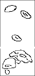
In this experiment, the test is performed on the same data set used in the previous experiments. Fig. 4 illustrates an example of 3 images from this data set. The mean values of FOM for the different edge detectors are summarized in Table 7.

Table 8. Execution times (msec) comparison

Image sizes (pixels)	Robert [40]	Canny [41]	Our algorithm
256×256	0.997	6.50	2.763
512×512	7.271	10.90	5.864
1024×1024	56.717	26.05	13.320

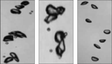
Fig. 4. Example of test images for the FOM assessment

Conclusion

In this paper, an effective method for accurate and real time edge detection based on the local variance of the input image was proposed. This algorithm is performed in two steps: in the first step, the local variance of each pixel is computed based on integral image, and then the resulting contours are thinning to generate the final edge map. Different implementations on Intel® core ™ i7-3770 CPU and Nvidia GPU Kepler architecture are tested using a set of synthetic and real images with different sizes. We have used CUDA to implement the algorithm on an NVIDIA GTX780 GPU, and compared its performances to the CPU implementation. Acceleration factors between 17× and 82× with different image sizes ranging from (128x128) to ( 1024x1024 ) pixels, have been reached with the GPU implementation compared to the CPU. Also, our algorithm was compared to the most commonly edge detection techniques existing in the literature, Robert and Canny in terms of results accuracy and computa-

tion time performance. A remarkably performance is reached with our algorithm. Our method is robust against changes of intensity contrast of edges and capable of giving high detection responses on low contrast edges. With such performances, accurately extraction of air bubbles boundaries in real-time becomes possible.