GPU-Based Volume Rendering for 3D Electromagnetic Environment on Virtual Globe

Published Online November 2010 in MECS

Electromagnetic environment (EME) is composed of natural and man-made electromagnetic radiation and this paper focuses on 3D visualization of man-made electromagnetic environment. EME is complicated and invisible, and it is difficult for users to decide how to plan and design the wireless systems because of a large number of wireless systems designed to serve a variety of commercial and military uses. Computer graphics can represent the numeric data vividly, through which users can intuitively understand the information that the numeric data implicates.

As EME is invisible, we represent it on the terrain by computer visualization and users can adjust parameters of electromagnetic devices to see their influence dynamically in time, so this approach provides excellent decision supporting and plan-aiding for users. But it is extremely difficult to represent 3D EME efficiently and accurately on terrain. In order to visualize the EME, we need to compute EME data using radio propagation model [1] [2] . Although finite difference time domain(FDTD) algorithm can accurately describe the propagation of

Manuscript received ; revised ; accepted Corresponding author: Chao Yang +8613786149482

electromagnetic wave, it fails to meet our needs of interactively and dynamically visualizing the EME in virtual battle space because of its time-consuming calculation. Longley-Rice radio propagation model(Irregular Terrain Model, ITM) [3] is a computerized method that could take into account the detailed terrain and atmosphere features. The model is based on electromagnetic theory and statistical analyses of both terrain features and radio measurements, and predicts the median attenuation of a radio signal as a function of distance. Because of the availability of digital terrain models (DTM) we can use the point-to-point prediction mode of the model to compute propagation losses due to terrain irregularity. This mode can predict the radio propagation in time, and it is suitable to visualize the EME on irregular terrain.

In our former works [4] , [5] , we implemented 3D representation of radar detection range on terrain based on isosurface rendering method, which only shows the outer boundary but fails to capture most of the volumetric information. Multiple transparent isosurface rendering [6] , [7] overcomes the single isosurface’s drawback by adding more information to rendered images. But it fails to clip the volumetric data and visualize the sectional information. Direct volume rendering (DVR) can overcome these drawbacks. DVR via 3D textures has positioned itself as an efficient tool for the display and visual analysis of volumetric data [8] . Thanks to the advances in graphics hardware performance and functionality, DVR using graphical processing units(GPU) [9] allows producing high quality rendering on current graphics hardware at interactive frame rates. GPU-based DVR which projects 3D volumetric data onto 2D image using front-to-back compositing is an important and popular technique used for volumetric data exploration. And it can show the inner detailed information of the volumetric data. So inheriting from [9] , we extend GPU-based DVR method to visualize the 3D EME on virtual globe, and propose an interactive method to show detailed information of EME at given place.

The paper is organized as follows: Section II is described the background of GPU-based DVR and general purpose computation on GPU; in section III, the framework of the GPU-based volume rendering system is proposed, and in section IV and section V, we will describe the GPU-based computation of 3D EME and extend GPU-based DVR on virtual globe in detail; The experiment results and conclusions are shown in section VI and section VII respectively.

• II.    BACKGROUND

Volume visualization is one of the important research fields in computer graphics. The recently works of GPU-based volume rendering is summarized in the book [10] . Here we only discuss the ray casting approach we relate to. Because of commodity graphics hardware fully programmable, traditional direct volume ray-casting rendering approach can completely transfer from CPU to programmable GPU, which can take advantage of parallel fragment units and high bandwidth to video memory. And GPU-based ray-casting can produce high quality 2D images on current graphics hardware at interactive frame rates. Now it is widely used in scientific visualization.

GPU-based ray-casting approach projects 3D volumetric data to 2D image along projecting direction. The rendering proxy mesh is a volume bounding box and its vertex color is assigned the 3D texture coordinates. And it is a multi-pass approach [8] , [9] to render the volumetric data. The first pass renders back faces of the volume bounding box to a 2D RGB texture by the performance of Frame Buffer Object(FBO) [11] . So the color components in the texture correspond to the termination point between the projecting rays of sight and volume. The second pass renders front faces of the volume bounding box. In this pass, the main ray-casting fragment shader is executed. In vertex shader, the vertex position is transformed to eye coordinates space and passed to fragment shader. In fragment shader, the termination point is fetched for each fragment from back faces texture by the transformed vertex position. So the projecting ray direction can be computed as fragment color minus termination point. And then the shader samples 3D texture of the volumetric data from front to back along the ray direction and assigns color to each sampler by the transfer function. At last it composes each sampler color along this ray direction as the final fragment color. The last pass is blended the 2D volume image to the scene. There are many methods to speed up the GPU-based ray-casting, such as octree [12] , early ray termination [13] , empty-space skipping [8] , and so on.

There are also many literatures on studying general purpose computation and visualization on GPU[17][18], such as cloud rendering[15] and fluid simulation[16]. Current GPU has high data bandwidth and high dense parallel computation, and it can render the pixel color to 3D texture, which can be used to calculate and output the 3D volumetric data directly. Therefore it enhances the application of the GPU in 3D volumetric data computation. Crane et al [19]proposed a real-time physically based simulation and rendering of 3D fluids. They showed not only how 3D fluids can be simulated and rendered in real time, but also how they can be seamlessly integrated into real-time applications. So inspired from [19], we use GPU to accelerate the 3D EME volumetric data computation, and output the volumetric data using 3D texture.

• III.    FRAMEWORK

This paper aims at exploiting graphics processing units (GPUs) for interactive volume rendering of 3D EME on virtual globe. The framework of the computation and rendering system is shown in Fig. 1. The steps in the dash box are run on GPU. The system consists of two major parts: GPU-based 3D EME calculation and direct volume rendering. Our system takes full advantage of the performance of current GPU.

The 3D EME computation is based on Longley-Rice radio propagation model(ITM). Using ITM, we can get power density of radio radiation at 3D space, while taking into account the effects of atmosphere and terrain. By calculating and summing the power density of every radio radiation within a certain frequency bands, the 3D EME volumetric data is constructed. All of these calculations are performed via a fragment shader. And the calculation result is stored in a 3D floating-point texture. We use the Ping-Pong technology [20] and bind different 3D textures to feed back the EME power density. To facilitate the use of GPU computing on 3D virtual globe, the 3D EME volumetric data is divided along the direction of latitude, longitude and height. Therefore, the resulting 3D floating-point texture uses spherical coordinate system for its voxels. The detail of GPU-based computation of 3D EME is described in section IV.

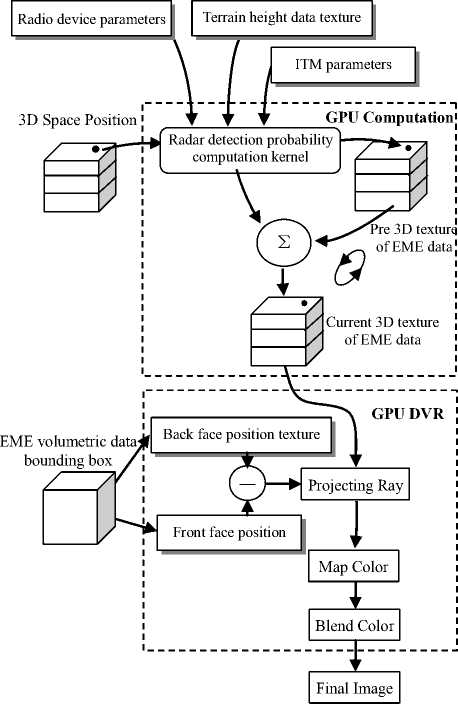
Fig. 1. System architecture

We use GPU-based DVR algorithm to render the 3D EME on virtual globe (detail in section V). Our DVR algorithm is similar to [9]. But the voxel position of the resulting 3D floating-point texture uses spherical coordinate system, and it is not regular. So the GPU-based ray-casting regular volume rendering approach can not be used to directly visualize the 3D EME volumetric data. We first transform the 3D EME volumetric data bounding box position to Cartesian coordinate, and then generate the projecting ray in Cartesian coordinate to sample the 3D EME power density data from the 3D texture. At the end, the map color is blended along the projecting ray to composite the final image. Through the coordinate transformation, the 3D EME volumetric data is directly rendered on virtual globe.

Because of using the GPU to accelerate, we can dynamically see the coverage of the 3D EME power density by adjusting the radio device parameters.

• IV.    Calculation of Power Volumetric Data of 3D EME

• A.    Calculating Propagation Loss

The ITM is used to calculate the 3D EME volumetric data. The purpose of the model is to estimate some of the characteristics of a received signal level for a radio link. This usually means cumulative distributions for what really appears to be a random phenomenon[14]. As described in an ESSA technical report[3], ITM model calculates path loss in three regions, called line-of-sight, diffraction, and scatter regions. And the reference attenuation Aref is determined as a function of the distance d from the piecewise formula:

A , ref

'max(0, Aei + K1 d + K 2ln( d / dh ), Aed + mdd, Aes + msd, d ^ dls

^dls ^ ^d ^ d x    (1)

d x ^ d

Where the coefficients A_el , K₁ , K₂ , A_ed , m_d , A_es , m_s , and the distance d_ls , d_x are calculated using the algorithms described in [14]. Free space propagation loss is:

L fs = 32.45 + 20lg f + 20lg d (2)

In which, f is the frequency of radio. So the propagation loss is:

L - L f + A ref

We use the radiated power density value of the radio to represent the EME. From (3), the radio radiated power density value in 3D space is:

P - P t - L - L_s

Where, P i is the power density of i th radio radiating at a certain place.

• B.    Profiles of Irregular Terrain

The point-to-point prediction mode of ITM requires terrain elevation database to extract terrain elevation profiles. We use the digital terrain elevation data (DTED). As shown in the left of Fig. 2, the red lines are the path between transmitter and receiver, and the blue lines are the DTED terrain. In order to extract the profile of terrain, we sample DTED along the path using bilinear interpolation. An example of profile of terrain is shown in the right of Fig. 2.

• C.    Calculating Power Volumetric Data

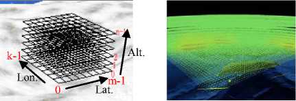
We suppose that there is a radio link between every radio and any 3D space position. Using (5), we can calculate 3D space radio power density value. But the original 3D space radio power density value is a large scale data field, it can not be used to visualize on terrain directly. So as shown in the left of Fig. 3, we divide the 3D space radio power density value into grids as follows. First, 3D space is divided into n layers along altitude direction, and then for each layer we divide it into m X k grids along longitude and latitude direction and calculate the radio power density value of every node in the grids. After all layers are processed, we will get a discrete 3D power density volumetric data, which is composed of m X kX n samples, as shown in the right of Fig. 3. So if there are N radio devices calculated on the virtual globe, the total number of radio links is m X k X n X N .

As described above, the calculation of 3D EME power density value is independent at each grid of divided volume space, so it’s suitable for parallel computing on GPU. We implement the computation as a fragment shader, and write the result to a 3D texture. Because GPU is designed to render to 2D frame buffer, we must execute fragment shader for each slice of the 3D texture. To run the fragment shader on a particular slice, we render a single quad whose size equals to the length and width of 3D volume. By running all slices along height, we can get the entire volumetric data.

Before the GPU calculation, we must input radio parameters (Position, Power, Gain, Frequency, System loss), and terrain height data into GPU. The radio parameters are organized as uniform structure and terrain height data is packed into a 2D texture. The output EME data is stored in two 3D textures which are bound to FBO by Ping-Pong technology. We swap the two 3D textures for output and input target. The pre 3D texture stores the summation of 3D EME power density of all radio devices before current radio device computing. The current 3D

In which, P t is the radio’s power, and L s is the other losses, such as system loss, operation loss.

If there are N radio devices within the frequency bands, the EME power density is summation of these N radio devices:

N

P-£ P i-1

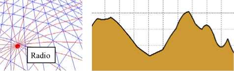
Figure 2. Extraction of terrain elevation profiles. Path between transmitter and receiver(left); profile of terrain(right)

• Figure 3. Construction of EME data field. Divided grids(left); power volumetric data of 3D space shaded in different colors on 3D globe(right)

texture stores the sum of power density of current radio device and pre power density from the pre 3D texture. When a radio device is finished calculating, the pre 3D texture and current 3D texture is exchanged for the next radio device computation.

The left of Fig. 4 shows the bounding box of 3D EME volumetric data which is from position minLLA ( lat 0 , lon 0 , alt 0 ) to position maxLLA ( lat 1 , lon 1 , alt 1 ) in spherical coordinates system. Where lat n , lon n , alt n ( n =0, 1) are latitude, longitude and height respectively. The resolution of computing bounding box is 256 X 256 X 64 which is determined by our GPU performance. We only compute the EME power density value within the bounding box. If required computing area is larger than the minLLA and maxLLA , the required computing area can be divided into appropriate bricks along the latitude and longitude direction. The area of terrain height texture covers position of all radio devices and the computing bounding box coverage and its resolution is 2048 X 2048. The terrain height profile can be looked up along the position from computing position to radio device at intervals of 1/2048. Therefore, we can extract the terrain elevation profile on GPU.

Here we summarize the approach of computing 3D EME power density value on GPU at a particular grid as follows:

• 1)    Input the radio device parameters, and the bounding box (minLLA, maxLLA);

• 2)    Transfrom the fragment position to spherical coordinate;

• 3)    Get pre summation of the power density from the pre 3D texture;

• 4)    Interpolate terrain profile from device postion to fragment position in the terrain texture;

• 5)    Use the ITM to calculate the current power density;

• 6)    Sum the pre power density and current power density, and output the summation to current 3D texture;

• 7)    Exchange pre 3D texture and current 3D texture for next one radio device computation.

rendering approach can not be used to directly visualize the 3D EME volumetric data. And in this section we extend the ray-casting approach to visualize the 3D power volumetric data of EME on globe and propose a method to show the detailed information of EME at given place interactively.

• A.    EME Volumetric Data Bounding Box

Fig. 4 shows the EME volumetric data bounding box on 3D globe and back faces texture. Suppose the 3D volumetric data is calculated in a bounding region from position minLLA( lat 0 , lon 0 , alt 0 ) to position maxLLA ( lat 1 , lon 1 , alt 1 ) in spherical coordinates system. Fig. 5 shows the 3D volumetric data in section using blue color. The volumetric data bounding box is marked by black wide lines. Obviously, the maximal altitude of volumetric data bounding box is alt 1 plus alt , and can be calculated as follows:

R + alt alt, + alt =       1 - R              (6)

• ¹          cos( ^ )

In which, R is the earth radius, 9 is equal to max( lat 1 - lat 0 , lon 1 - lon 0 )/2, so the volumetric data bounding box is larger than volumetric data calculating region(see Fig. 5).

In GPU-based ray-casting rendering approach, the 3D texture coordinates are assigned as color to each vertex of the volumetric data bounding box, which is rendered to a back faces texture as projecting ray termination point. But the 3D EME volumetric data is not regular grid; it’s difficult to get its 3D texture coordinates at each vertex of bounding box. Furthermore, the 3D texture coordinates can not be directly assigned to vertex, because the texture coordinates system is not homogeneous in the bounding box. We propose a novel method which does not assign 3D texture coordinates to each vertex directly, but uses vertex’s position of spherical coordinates and transforms spherical coordinates to texture coordinates in fragment shader. Because the spherical coordinates are not homogeneous, first the spherical coordinates are transformed to Cartesian coordinates as follows:

x = R cos( a )cos( e )

< y = R cos( a ) sin( в ) (7)

z = R sin( a )

Where, R, а,в are spherical coordinates; x , y , z are Cartesian coordinates. Using (7), the eight vertexes’ position of volumetric data bounding box are transformed to Cartesian coordinates which are assigned as color to the

V. Volume Rendering EME on 3D Globe

In section II, we revisited GPU-based ray-casting volume rendering approach, which visualizes regular volumetric data and uses regular volume bounding box as proxy mesh. 3D volumetric data of EME calculated using the method described in section IV is not regular, and the volumetric data is organized in spherical coordinates system. So the GPU-based ray-casting regular volume

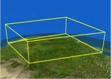
Figure 4. EME volumetric data bounding box. Wireframe of bounding box(left); back faces texture of bounding box(right)

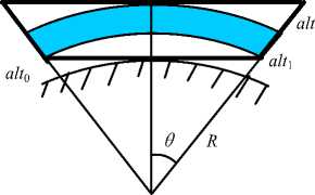
Figure 5. Section of volumetric data bounding box(wide lines), filled color parts is the volumetric data

vertexes. And then by the performance of floating point texture, the floating color value of volumetric data bounding box can be rendered to texture. So the fragment shader can fetch the floating Cartesian coordinates from this texture as projecting ray termination point.

• B.    Volumetric Texture Coordinates Transformation

In our approach, each vertex’s color of volumetric data bounding box is its vertex’s Cartesian coordinates position. By rendering the back faces of bounding box to floating point texture as projecting ray termination point and rendering the front faces as projecting ray start point, the projecting ray direction is calculated in fragment shader using vector difference between projecting ray termination point and start point. Traveling along the projecting ray direction, fragment shader is able to fetch EME value from the volumetric texture which contains the volumetric data. But projecting ray is in Cartesian coordinates system, and it needs to transform to texture coordinates system to fetch value from texture. Because the volumetric texture’s bounding box is from position minLLA ( lat 0 , lon 0 , alt 0 ) to position maxLLA ( lat 1 , lon 1 , alt 1 ) in spherical coordinates system, the texture coordinates of this sampling point can be interpolated by spherical coordinates with texture’s bounding box.

Transformation of Cartesian coordinates to spherical coordinates is:

R = V x 2 + У 2 + z 2

< a = arcsin ( z/R )                          (8)

в = arctan ( y/x )

Interpolation of texture coordinates is:

a - latо lati - latо в - lonо loni - lonо

R — alt о alt i - alt о

The valid range of the volumetric texture coordinates u , v , s is from 0 to 1. So if the volumetric texture coordinates are beyond the valid range, empty-space skipping method can be used to speed up the volumetric data rendering.

The pseudo-fragment shader of our DVR algorithm is that:

float4 fragColor = {0, 0, 0, 0};

float3 vecStart = fragmentposition;

float3 vecTermin =

GetFromBackFacesTexture(fragmentposition); float3 vecRayDir = vecStart – vecTermin;

for(i = 0 to n segments)

{ float3 samplepos = TransformTextureCoord(i, vecRayDir);

//Clip volume data if(samplepos is in clip area) continue;

float EMEdensity =

GetDensityfrom3Dtexture(samplepos);

fragColor.a = color.a + fragColor.a * (1 -color.a);

} return fragcolor;

• C.    Detail Information Widget

The 3D EME is represented using GPU-based volume ray-casting rendering approach. Although it shows the situation of EME composed of many wireless systems on 3D space, it fails to get the detail information of every single wireless system radiation from the volume rendering result, which is important for wireless systems design. The detail information widget is proposed to meet the needs. As shown in Fig. 6, the detail information widget is composed of selected arrows, information box and connected line. The origin of selected arrows represents 3D space position of querying detail information, and the arrows can be picked and moved along latitude, longitude, altitude direction by mouse cursor. The detail information of EME at the origin of selected arrows can be shown immediately in the information box which lists all wireless systems of EME. The wireless system can be selected in the information box marked by white rectangle, and it is connected to the origin of selected arrows by a white line which shows the distance between selected wireless system and information querying position. So with our novel detail information widget, the radiation of every wireless systems of EME is shown in detail at any position of virtual globe interactively.

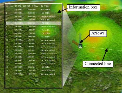
Figure 6. Detail information widget

• VI.    Experiment Results

  The prototype system is implemented using OpenGL and Cg in the Windows operation system. In our experiments, twenty radio devices are located on the virtual globe which has a latitude-longitude grid spacing of 30 arc-seconds terrain data. These radio devices’ parameters are shown in Table I. The polarization is horizontal. The parameters of ITM propagation model are that surface refractivity is 320 N-units, and dielectric constant and conductivity of ground is 15 and 0.005 S/m respectively. The experiments are run on an Intel Pentium Dual 1.8 GHz (2 GB) with a GeForce 8600 GT graphic card (256 MB).

Fig. 7 shows the volume visualization of EME on 3D globe. The volumetric data has a resolution of 256 X 256 X 64 with 32 bits/sample. If the volumetric data is larger, the volumetric data can be divided into several bricks with appropriate size. Each brick is rendered by our ray-casting approach, and then every bricks are blended from back to front. So our approach is suitable for visualizing large EME volumetric data on 3D globe.

TABLE I. P arameters of radio devices

Device No	Frequency (MHz)	Power (kw)	Gain (dB)
1	450	2500	20
2	200	2500	15
3	500	3000	18
4	350	1500	25
5	320	2000	22
6	200	1500	26
7	500	1200	17
8	400	1200	26
9	500	2000	21
10	100	500	15
11	200	100	21
12	350	500	18
13	350	600	26
14	300	2500	18
15	480	500	30
16	200	1000	21
17	350	450	32
18	350	2500	18
19	400	1500	20
20	500	1200	29

T able 2 C omparison between CPU and GPU

Volume size	Calculation(s)
	CPU	GPU
128×128×64	32	0.98
256×256×64	132	3.64

From Table 2, we can see that GPU based implementation improves the computing performance about 30 times than the CPU based. Our GPU based system is able to interact in real-time. And the average rendering frame rate is 25fps with a widow size of 1024 X 768.

The EME is represented by interactively assigned different color and opacity with color picker(see bottom of Fig. 7). The EME coverage affected by irregular terrain is vividly and dynamically visualized in time and the parameters of radios can be adjusted interactively, which can provide excellent decision supporting and plan-aiding for users. The top left of Fig. 7 is the result of closing one radio marked by a white circle in the lower-right corner, and it’s clearly and intuitively to see how much the coverage decreases. As shown in Fig. 8, the inner information of EME can be represented by clipping the volumetric data. The 3D EME volumetric data is clipped in altitude, longitude, and latitude direction respectively. So the inner detail information can be seen, and our method can supply more information than isosurface rendering.

• VII.    CONCLUSIONS

We have proposed an approach to extend the GPU-based DVR to represent EME on virtual globe at interactive frame-rates. The Longley-Rice radio propagation model(ITM), which takes into account the effects of irregular terrain and atmosphere, is used to calculate the power density volumetric data. And we use GPU to accelerate the ITM computation. We also present

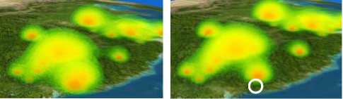
Figure 7. Rendering results. (Top right) is closed one radio marked by white circle from(Top left); (bottom) is color picker.

Figure 8. Clipping volumetric data. EME at altitude of 500m(left) and 5000m(middle); clipping along longitude and latitude direction(right) a widget to interactively show detailed information of EME at given place. At last, the interactive 3D EME visualization is implemented on virtual globe, and the results show that this approach can represent the 3D EME at interactive frame rates. Moreover, the EME coverage is vividly and dynamically visualized in time and parameters of radios can be adjusted interactively, which can provide excellent decision supporting and plan-aiding for users.

Although we use ITM to calculate the power density of the 3D EME, it‘s difficult to validate the results to the real 3D EME. Because the radio radiation is influenced by terrain, atmosphere, weather, jamming, and other electromagnetic devices, and different areas have different states. Only the terrain and atmosphere influence are statistical considered in the ITM, and many complicated cases were not considered. If all the cases can be modeled, the predicted result would be more accurate. We have only advanced a half step on the way of representing 3D EME accurately. Next we set out to do some work on computation so as to represent a more accurate EME coverage. At the same time more representing manners are also our aspiration. We plan to extend our approach to support large-scale volumetric data, and optimize the EME calculation.

Acknowledgment

The authors thank the anonymous reviewers for their helpful comments, and thank all the people at Institute for Telecommunication Sciences for their wonderful work on ITM. This work is supported by the National High Technology Research and Development Program of China (863 Program) under Grant No. 2009AA01Z335.