Graph Neural Networks for Predictive Maintenance in IoT Sensor Systems Using Device Telemetry Data

The rapid expansion of the Internet of Things (IoT) has transformed industrial environments by enabling continuous monitoring of machines through interconnected sensors and embedded devices. These systems generate high-frequency telemetry data, such as temperature, vibration, pressure, and voltage readings, which provide critical insights into equipment health. Predictive maintenance leverages this data to anticipate failures before they occur, reducing downtime, maintenance costs, and safety risks. Unlike reactive or scheduled maintenance, predictive maintenance depends on intelligent data-driven models capable of detecting subtle degradation patterns. However, IoT sensor data are high-dimensional and inherently spatio-temporal, as devices interact within structured networks. Conventional machine learning methods often struggle to capture such relational dependencies. Graph Neural Networks (GNNs) address this limitation by modelling sensors as nodes and their interactions as edges within a graph structure. When combined with temporal modelling techniques, these approaches capture both structural relationships and sequential degradation behaviour, enabling scalable and reliable predictive maintenance in modern IoT-driven industrial systems [1].

Regression and classification in predictive maintenance rely on deep learning frameworks designed for multivariate time-series analysis. Preprocessing typically includes noise filtering, missing value handling, and normalization. Feature engineering extracts statistical indicators and degradation-related signals to represent equipment behaviour. Convolutional and recurrent neural networks are commonly applied to identify fault patterns and categorize machine states into normal or faulty conditions [2]. More recently, GNNs have been used to capture spatial dependencies among interconnected sensors, while BiLSTM networks model temporal dynamics. Attention mechanisms enhance performance by prioritizing informative features and relationships. Multi-task learning frameworks enable simultaneous fault classification and Remaining Useful Life (RUL) estimation, improving generalization and computational efficiency through shared representations within IoT-based maintenance systems. Existing Regression and classification frameworks have improved early fault detection and RUL prediction accuracy [3]. Deep learning models incorporating temporal and attention mechanisms generally outperform traditional statistical approaches in capturing complex degradation patterns. Graph-based methods enhance representation of sensor interdependencies, improving fault localization and classification consistency across distributed IoT networks. Multitask learning further boosts predictive performance by sharing features between classification and regression objectives. Evaluation metrics such as accuracy, precision, recall, F1-score, RMSE, and MAE demonstrate reduced false alarms and more reliable failure estimation. These advancements support optimized maintenance scheduling, cost reduction, and scalable deployment in smart manufacturing environments [4]. Overall, integrating spatial–temporal modelling with graph learning enhances robustness and operational efficiency in IoT-driven predictive maintenance frameworks.

Despite these advancements, several challenges remain. IoT telemetry data are often noisy, incomplete, and imbalanced, affecting model reliability. Labelled failure data are limited in real-world settings due to the rarity of faults. Static graph construction may not reflect dynamic sensor relationships, reducing adaptability [5]. Temporal models like BiLSTMs may struggle with very long or non-stationary sequences, and multi-task learning can face task interference between objectives. Scalability and computational complexity are concerns for large-scale IoT deployments. Additionally, limited model interpretability restricts practical adoption, as engineers require transparent decision support. Addressing these issues requires adaptive graph construction, robust feature extraction, efficient training strategies, and explainable architectures to ensure reliable real-world deployment.

The proposed method introduces a hybrid Graph Attention Network–Long Short-Term Memory (GAT–BiLSTM) framework within a multi-task architecture for predictive maintenance using IoT telemetry data [6]. After preprocessing and feature extraction, a dynamic graph construction module defines sensor nodes and interdependencies through an adjacency matrix. The GAT component models spatial correlations via attention-weighted message passing, assigning adaptive importance to neighbouring sensors. A BiLSTM encoder captures temporal degradation trends and long-term dependencies. A spatio-temporal fusion layer integrates spatial and temporal embeddings into a unified representation. The framework employs dual output heads: a classification head for fault detection and probability estimation, and a regression head for RUL prediction. This shared-learning design enhances generalization while reducing redundant computation. The integration of adaptive graph attention with temporal modelling aims to improve early fault detection accuracy and provide reliable RUL estimation in complex IoT sensor networks [7]. The key contributions of this work are summarized as follows. First, we propose a dynamic graph-based predictive maintenance framework that captures evolving relationships among sensor nodes, unlike static graph approaches used in conventional GAT-BiLSTM models. Second, we introduce a cross-attention mechanism that enables effective interaction between temporal and spatial features, improving feature representation quality. Third, a gated fusion strategy is designed to adaptively combine multi-source information, enhancing robustness to varying operational conditions. Fourth, a multi-task learning formulation is employed to jointly optimize fault classification and prediction objectives, improving overall performance. Compared to existing hybrid spatio-temporal models, the proposed approach provides better adaptability, feature interaction, and generalization capability.

This paper is structured as follows. The Introduction outlines the research background and objectives. The Literature Survey reviews existing predictive maintenance approaches and identifies research gaps. The Proposed Method describes the GNN-based architecture and modelling strategy. The Results and Discussion section evaluates experimental performance using standard metrics. Finally, the Conclusion summarizes contributions and future directions, followed by the References.

2.    Literature Survey

The field of Graph Neural Networks for Predictive Maintenance in IoT Sensor Systems has gained significant attention due to the increasing deployment of interconnected sensors in industrial environments. Accurate fault detection, degradation modelling, and Remaining Useful Life estimation are essential for reducing downtime and optimizing operational efficiency. Recent years have witnessed rapid growth in research efforts, characterized by diverse methodologies including graph-based learning, spatio-temporal modelling, attention mechanisms, and hybrid deep learning frameworks. This literature survey systematically reviews existing approaches to identify technological advancements, methodological trends, persistent challenges, and critical research gaps guiding future developments.

This category includes studies primarily focused on graph-driven or machine learning–based fault classification. Elkateb et al. [8], propose an IoT-enabled predictive maintenance system using ESP32 sensors combined with an AdaBoost classifier optimized via Grid Search to identify machine stoppage causes. While achieving 92% accuracy, the approach requires expanded datasets to generalize across machines. Li et al. [9], introduce a Filter-informed Spectral Graph Wavelet Network (SGWN) that extracts multiscale spectral features for fault diagnosis, mitigating oversmoothing in deep GNNs; however, interpretability depends heavily on domain-specific fault mechanisms. Atticus et al. [10], design a GNN framework for reliability prediction in smart infrastructure, leveraging message passing for node-and edge-level classification, yet performance declines with sparse graphs and large-scale computational demands. Wang et al. [11], develop a Multi-level Spatiotemporal GNN (MLS-GNN) integrating GAT and adaptive thresholding for wind-powered heating fault detection, though high computational complexity and limited fault samples constrain deployment. Collectively, these studies demonstrate the strength of graph-based classification in modelling interdependencies, while highlighting challenges related to scalability, data quality, interpretability, and computational overhead in real-world IoT environments.

This category focuses on regression-oriented frameworks that model temporal dynamics and graph dependencies. Niresi et al. [12], propose the Spatial-Temporal Graph Attention Fuser (STGAT-Fuser), integrating 1D convolution, GATv2 layers, and BiLSTM modules to improve multisensory calibration accuracy. Although effective, further exploration across domains and architectures is required. Sharma et al. [13], introduce Equi-Euler GraphNet, a physics-informed, equivariant GNN using Euler-based temporal updates to predict forces and trajectories in multi-body systems, achieving strong extrapolation but lacking real-world experimental validation. Topu et al. [14], present a Digital Twin-driven GNN for pavement health forecasting, modelling road segments as graph nodes with real-time data streams; however, moderate distress classification remains challenging, and computational demands are high. These regression-focused approaches emphasize dynamic graph modelling and temporal reasoning to predict continuous variables such as degradation levels, calibration errors, or physical states. Despite promising accuracy and efficiency improvements, they commonly face limitations in generalization, data sparsity, and validation under real operational conditions, underscoring the need for robust, scalable, and experimentally verified regression frameworks in predictive maintenance.

This category encompasses hybrid architectures that jointly address classification and regression tasks. Chen et al. [15], propose a multi-sensor fusion model combining Graph Attention Networks with cross-modal Transformer decoders, enabling simultaneous Remaining Useful Life (RUL) regression and tool health classification through a dualhead structure. While demonstrating significant MSE and MAE reductions, the framework depends heavily on flank wear indicators and incurs high computational costs. Wang et al. [16], (MLS-GNN) also integrate classification and regression objectives, capturing dynamic thermoelectric coupling with adaptive thresholding, yet face scalability and lightweight deployment issues. Atticus et al. similarly incorporate node-level classification and edge-level risk regression within infrastructure graphs, though sparse connectivity can hinder learning. These hybrid models leverage shared spatio-temporal representations to enhance predictive consistency and reduce redundant training. However, multi-task interference, increased architectural complexity, and resource-intensive training remain recurring challenges. Overall, hybrid graph frameworks reflect a growing trend toward unified predictive maintenance systems capable of simultaneously diagnosing faults and estimating degradation severity.

This category includes algorithmic frameworks integrating reinforcement learning and optimization for maintenance decision-making. Qiu [16] proposes an MDP-based architecture combining Fourier Neural Operators for temporal modelling, Denoising Autoencoders for robust state representation, Graph Neural Networks for relational modelling, and Proximal Policy Optimization (PPO) for optimal maintenance policy learning. Although achieving reduced long-term maintenance costs, the framework exhibits high memory usage, inference delays, and limited validation on real datasets. Varalakshmi et al. [17], develop a deep reinforcement learning and ensemble-based framework integrating DRL, Random Forest, and Gradient Boosting for adaptive fault detection and scheduling in streaming IIoT environments. Despite high classification performance, reliance on synthetic data and limited evaluation on edge devices restricts real-world applicability. These optimization-driven approaches shift predictive maintenance from pure fault detection toward prescriptive decision-making, enabling adaptive policy learning under dynamic conditions. However, their complexity, interpretability concerns, computational requirements, and dependence on simulated environments highlight the need for lightweight, explainable, and experimentally validated reinforcement learning strategies in industrial IoT systems.

3.    Proposed Method

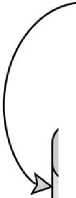
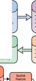
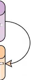
The proposed architecture (Fig. 1) integrates dynamic graph construction with a GAT–BiLSTM spatio-temporal network, enabling adaptive spatial learning and bidirectional temporal modelling for joint fault classification and RUL estimation.

The proposed framework (Fig. 1) presents an end-to-end intelligent monitoring and prediction pipeline designed for condition assessment and fault prognosis in complex systems. The architecture integrates signal preprocessing, feature engineering, dynamic graph modelling, and a hybrid deep learning backbone combining Graph Attention Networks (GAT) and Bidirectional Long Short-Term Memory (BiLSTM) to capture spatial dependencies and temporal dynamics simultaneously. The system ultimately performs multi-task predictions, including failure probability estimation, fault classification, and Remaining Useful Life (RUL) regression, supported by comprehensive performance evaluation metrics. The pipeline begins with raw data acquisition, followed by a pre-processing stage that enhances data quality through noise filtering, missing value imputation, and outlier removal. This stage ensures robustness by reducing measurement errors and improving statistical reliability. The cleaned data proceeds to the feature engineering module, where statistical descriptors, health indicators, spectral features, and degradation trends are extracted. This multi-domain representation enables the model to capture both steady-state behaviour and progressive deterioration patterns. Next, a dynamic graph construction module transforms feature vectors into a relational structure. Nodes represent system components or sensor channels, while edges are formed using k-nearest neighbour (kNN) relationships. Edge weights are dynamically updated based on similarity measures, and an adaptive adjacency matrix enables the graph topology to evolve with system state changes. This design allows spatial dependencies and component interactions to be explicitly modelled.

Dynamic Graph Construction

• Sensor Nodes

• Edge Weights

• Graph Topology Discovery

1. Vibration (x,y,z)

2. Temperature

3. Pressure

4. Acoustic Emissions ^5. Current/Voltage

Raw loT Sensor Telemetry

Sensor Nodes Edge Weights (Similarity) • Graph Topology Discovery

* Multi-Head

• Feature Aggregation

• Node Embedding

BiLSTM Temporal Model

Data Preprocessing

Graph Attention Network (GAT)

Dynamic Graph Construction

• Noise Reduction

• Normalization

• Missing Value Imputation

■ Outlier Detection

Feature Engineering

Dataset Preparation

Representation

• •    Forward LSTM

• •    Backward LSTM

• •    State Concatenation

Temporal Feature Representation

• •    Cross-Attention Mechanism

• •    Gated Feature Integration

• •    Adaptive Weighting

■ Time-Domain Features

■ Frequency-Domain Features

• Time-Frequency Features

• Statistical Aggregation

Sliding Window Segmentation Sequence Labelling

• Train/Val/Test Split

Shared SpatioTemporal Representation

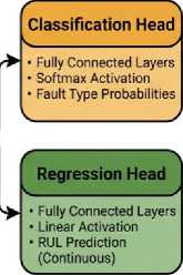
Fig. 1. Dynamic GAT–BiLSTM Multi-Task Predictive Maintenance Framework.

The core learning engine is the GAT-BiLSTM Spatio-temporal network, which operates through parallel branches. The GAT branch performs edge-weighted feature updates and neighbourhood aggregation via attention-based message passing, capturing spatial correlations. The BiLSTM encoder processes sequential data in forward and backward directions, extracting temporal context and long-term dependencies. A cross-attention and gated fusion layer integrates spatial and temporal representations, followed by residual fusion to preserve low-level information and stabilize training. The fused representation feeds multi-task prediction heads. A classification head estimates failure probability and fault categories, while a regression head predicts RUL. Parallel evaluation metrics (accuracy, precision, recall, F1-score, RMSE, MAE, R², and MAPE) quantify both classification and prognostic performance. The modular design supports parallel processing of spatial and temporal features, adaptive graph updates for evolving system behaviour, and multiobjective learning. These design choices enhance interpretability, predictive accuracy, and robustness in real-world condition monitoring environments. The pre-processing module ensures data reliability and consistency before feature extraction and modelling. Its inputs consist of raw sensor signals or operational measurements that may contain noise, missing entries, and extreme outliers. Noise filtering is applied using smoothing filters or frequency-domain denoising methods to remove high-frequency disturbances and measurement artifacts. Missing value imputation techniques such as mean substitution, interpolation, or model-based imputation reconstruct incomplete observations while preserving temporal continuity. Outlier removal is performed using statistical thresholds (e.g., z-score or IQR methods) to eliminate anomalous values that could distort downstream learning. This module transforms raw measurements into clean and standardized data suitable for feature extraction. It improves model stability and prevents bias caused by corrupted readings. The outputs feed directly into the feature engineering stage, ensuring consistent statistical distributions. By improving signal quality and removing anomalies, this block enhances generalization performance and reduces sensitivity to measurement noise common in industrial environments.

The feature engineering module converts cleaned signals into informative descriptors that characterize system behaviour and degradation. Inputs consist of pre-processed time-series data. Statistical features (mean, variance, skewness, kurtosis) summarize distributional properties. Health indicators are derived from domain knowledge to quantify component condition. Spectral features extracted using Fourier or wavelet transforms capture frequencydomain characteristics indicative of wear or imbalance. Degradation trend features track long-term performance decline through slope estimation or moving averages. The module transforms raw signals into a compact multi-domain feature vector that reflects operational state, dynamic behaviour, and deterioration patterns. These features enhance model interpretability and allow early fault detection by highlighting subtle deviations from normal behaviour. The outputs serve as node attributes in the graph construction stage, enabling relational learning. Combining time, frequency, and trend-based descriptors provides a comprehensive representation, improving prediction robustness under varying operating conditions. This module builds an adaptive relational structure to capture dependencies among system components. Inputs include engineered feature vectors representing sensors or subsystems. Each node corresponds to a component, while edges are constructed using k-nearest neighbour (kNN) similarity based on feature distance metrics such as Euclidean or cosine distance. Edge weights reflect similarity strength and are dynamically updated as system behaviour evolves. An adaptive adjacency matrix enables the graph structure to change over time, allowing the model to capture shifting relationships due to operational changes or progressive faults. This dynamic representation improves sensitivity to emerging anomalies and component interactions. The graph serves as input to the GAT branch, where attention mechanisms exploit connectivity patterns for spatial feature aggregation. By modelling interdependencies explicitly, this module enhances fault localization and improves prediction accuracy in interconnected systems.

The hybrid spatio-temporal network forms the analytical core of the system. The GAT branch processes the dynamic graph by applying attention mechanisms to compute edge-weighted feature updates and neighbourhood aggregation. This message-passing process enables each node to incorporate contextual information from its neighbours while learning the relative importance of connections. Simultaneously, the BiLSTM encoder processes sequential node features to model temporal dependencies. Forward and backward passes capture both past and future context, while a temporal attention layer emphasizes critical time steps. A cross-attention mechanism aligns spatial and temporal representations, and a gated fusion unit adaptively combines them. Residual fusion preserves original features and stabilizes gradient flow. The fused representation encodes spatial correlations and temporal evolution, making it suitable for prognostics and fault diagnosis. This architecture leverages parallel processing and attention-based weighting to improve interpretability and performance.

The prediction module performs simultaneous classification and regression tasks using the fused spatio-temporal representation. The classification head estimates failure probability and identifies fault classes through fully connected layers and softmax activation. The regression head predicts Remaining Useful Life (RUL), enabling predictive maintenance scheduling. Multi-task learning allows shared feature representations to improve generalization while reducing computational redundancy. Performance is evaluated using classification metrics (accuracy, precision, recall, F1-score) and regression metrics (RMSE, MAE, R², MAPE). These metrics provide complementary insights into diagnostic accuracy and prognostic reliability. The failure probability output can also serve as feedback to the RUL regression head, enabling risk-aware life prediction. This integrated evaluation framework ensures comprehensive system assessment and supports decision-making in maintenance planning.

• 3.1.    Input Representation and Preprocessing

X = {x1,x2,^,xT},xte^!1                                    (1)

The multivariate time-series input is denoted as X, where ^represents the number of time steps and (/corresponds to the dimensionality of sensor features. Each observation x _t captures system behavior at time t, forming the basis for downstream processing.

X pre =P(X)

where P(-)denotes preprocessing (noise filtering, missing value imputation, and outlier removal).

• 3.2.    Feature Engineering

F t = Ф(X pre,t )

where Ф(•)extracts statistical, spectral, and degradation features.

F = {F1,F2’^’Ft]

The sequence Frepresents the processed feature set over time. It serves as the input for both graph-based spatial modeling and temporal sequence learning modules.

• 3.3.    Dynamic Graph Construction

G t = (V_eE_eAt)                                            (5)

where Vt denotes nodes, Etedges, and Atthe adaptive adjacency matrix.

A" = {exp ⁽

И F - F i ||²

O'2

0,

■),  if jeNk(i), otherwise.

where Nte(i)denotes the к-nearest neighbors.

• 3.4.    Graph Attention Network (GAT)

h^(i+l) = ^ ( ^^ ^a ii Wh -" ) \iSN_t          /

The GAT layer updates node embeddings by aggregating features from neighbouring nodes using attention weights. This mechanism enables selective focus on the most informative relationships in the graph.

exp (LeakyReLU(d^T[Wh[ || Wh / ]))

^aii   S fceWj exp (LeakyReLU(a^T[Wh , H Wh_te]))

The attention coefficients a^ quantify the importance of node jto node i . They are normalized using a softmax function to ensure proper weighting across all neighbours.

• 3.5.    BiLSTM Temporal Modelling

• 3.6.    Cross-Attention Mechanism

  Attention(Q'K'V) = Softmax

  
  

  (I

  
  

  V

  
  
  
  

ht = LSTMf0rward (Ft, ht_)(9)

The forward LSTM processes the sequence in chronological order, capturing dependencies from past observations. It provides a representation that reflects historical trends in the data.

К = LSTMbackward (^ K+l)

The backward LSTM processes the sequence in reverse order, incorporating future context into the representation. This enhances the model’s understanding of temporal dependencies.

Ht = [к и K](ii)

The final temporal representation is obtained by concatenating forward and backward hidden states. This bidirectional encoding provides a comprehensive temporal feature vector.

The cross-attention mechanism facilitates interaction between spatial and temporal features. It computes attention scores using query, key, and value matrices to capture interdependencies across modalities.

• 3.7.    Gated Fusion Mechanism

• 3.8.    Multi-Task Learning Objective

g = a(Wg[Hs\\Ht] + bg)(13)

The gating vector gcontrols the contribution of spatial and temporal features. It is learned adaptively to balance information flow based on input characteristics.

Hfusion =gOHs + (1-g)OHt

The fused representation combines GAT and BiLSTM outputs using element-wise weighting. This enables robust feature integration and improves representation quality.

Pciass = Softmax(WcHfuSion + bc)

The classification head output’s fault class probabilities using a SoftMax function. It enables the model to distinguish between different fault categories.

^^^ pred = ^Wr^Hfusion ^{+ b} r

The regression head predicts the Remaining Useful Life (RUL) as a continuous value. This supports predictive maintenance decision-making.

• 3.9.    Loss Function

  L = A₁L cis

  
  

  + ^ 2^Lreg

  
  
  
  

The total loss function combines classification and regression objectives. The weighting factors A1and Л2 control their relative importance.

L cis =—Ey i log(P i )                                          (18)

The classification loss is computed using cross-entropy, measuring the discrepancy between predicted and true class labels. It ensures accurate fault classification.

L

reg = 1 ^(^y ^L _t rue

² ^^ ^Lpred J

The regression loss is defined as mean squared error between predicted and true RUL values. It penalizes large deviations and improves prediction accuracy.

4.    Result and Discussion

The proposed predictive maintenance model was implemented in Python using the Google Colab environment, leveraging an NVIDIA A100 GPU for accelerated computation. The setup provided an efficient platform for training deep neural networks, enabling high-performance processing of IoT telemetry sequences and ensuring optimal utilization of computational resources for model optimization.

• 4.1.    Model Specification

• 4.2.    Datasets

• 4.3.    Classification Metrics

The proposed model adopts a hybrid Graph Attention Network–Long Short-Term Memory (GAT–BiLSTM) architecture within a multi-task learning framework for predictive maintenance using IoT telemetry data. Initially, sensor measurements are preprocessed and organized into temporal windows to capture sequential behaviour. A dynamically constructed graph represents sensors as nodes and their interactions as edges, enabling structured relational modelling. The Graph Attention Network module, composed of two layers with multi-head attention, learns spatial dependencies by assigning adaptive importance weights to neighbouring sensors. The extracted spatial embeddings are then forwarded to a stacked BiLSTM network that models long-term temporal degradation patterns and sequential dependencies. A spatio-temporal fusion layer integrates graph-based and temporal features into a unified representation. The network employs dual output heads: a classification head for fault detection and a regression head for Remaining Useful Life estimation. Joint optimization using a weighted multi-task loss enhances generalization, reduces redundant computations, and improves overall predictive performance in IoT-based industrial systems. The proposed model introduces additional computational overhead due to the integration of GAT, BiLSTM, and attention mechanisms. The overall complexity is approximately O(N2) for graph construction and attention computation. However, this cost is justified by improved predictive performance. Optimization techniques such as sparse graph representation and model pruning can be applied to improve scalability. Table 1 summarizes the architectural and training parameters of the GAT-BiLSTM model employed in this study. It outlines the core backbone configuration, embedding and attention settings, and optimization strategy, highlighting the model’s suitability for IoT telemetry representation and predictive maintenance tasks.

Table 1. Parameter Specification of GAT-BiLSTM.

Parameter	Value Set
Number of GAT Layers	2
Dropout Rate (GAT)	0.3
BiLSTM Layers	2
BiLSTM Hidden Units	128
Sequence Length	50 time steps
Learning Rate	0.001 (Adam optimizer)
Batch Size	64
Multi-Task Loss Weight	1.0 : 0.5
Parameter	Value Set
GAT Hidden Units	64
Number of Attention Heads	4

For real-world deployment, factors such as latency, scalability, and robustness must be considered. The proposed model can be adapted for edge deployment using lightweight architectures and model compression techniques. Additionally, the framework is designed to handle missing or noisy sensor data through robust feature learning and adaptive fusion strategies.

The performance of the proposed classification model is quantitatively assessed using standard evaluation metrics derived from the confusion matrix. These metrics measure the model’s capability to correctly distinguish between positive and negative classes.

TP + TN

Accuracy =

1 TP + TN + FP + FN

The accuracy represents the proportion of correctly classified samples over the total number of samples, providing an overall measure of model correctness.

TP

Recall = —--—

TP + FN

The recall (sensitivity) measures the ability of the model to correctly identify positive instances, indicating how well actual positives are detected.

TP

Precision =

TP + FP

The precision metric indicates the proportion of true positive predictions among all predicted positive samples, reflecting prediction reliability.

TN

Specificity =

TN + FP

The specificity quantifies the proportion of actual negative samples correctly classified, measuring the model’s ability to avoid false alarms.

2 • (Precision • Recall) F1-score =

Precision + Recall

The F1-score represents the harmonic mean of precision and recall, providing a balanced evaluation when class distribution is uneven.

AUC = ( T P R(F PR - ^x)) dx о

The Area Under the Curve (AUC) evaluates the classifier’s ability to distinguish between classes across different threshold values, summarizing overall performance.

Here, TP, TN, FP, and FNdenote true positive, true negative, false positive, and false negative counts, respectively. TPRand FPRrepresent true positive rate and false positive rate. The superior performance of the proposed model can be attributed to its ability to effectively capture both spatial dependencies through graph attention and temporal dynamics via BiLSTM. The cross-attention mechanism enhances feature interaction, allowing the model to focus on critical patterns. Performance improvements are particularly noticeable under complex fault conditions, where traditional models fail to capture evolving dependencies.

As shown in Table 2, classification results for each class yield competitive F1‑Score, specificity, sensitivity, accuracy, Dice coefficient and precision metrics.

Table 2. Performance of classification based on each class.

Classes	F1 Score	Spe	Sen	Acc	Dsc	Precision
Failure probability	0.991	0.994	0.995	0.995	0.991	0.988
Fault class	0.996	0.995	0.994	0.995	0.996	0.968

As shown in Fig. 2, the confusion matrix illustrates the classification performance of the proposed model, achieving 1493 true positives and 3482 true negatives with minimal misclassifications, demonstrating high detection reliability and balanced fault identification capability.

The proposed GAT‑BiLSTM model outperforms existing approaches in terms of accuracy, precision, F1‑score, and AUC, demonstrating superior classification reliability and generalization capability for predictive‑maintenance tasks. As shown in Table 3, quantitative results illustrate that our GAT‑BiLSTM achieves 0.995 accuracy, 0.988 recall, 0.995 precision, 0.991 F1‑score and 0.997 AUC, surpassing other competing schemes. As shown in Fig. 3, (a) Accuracy, (b) Recall, and (c) Precision comparisons demonstrate that the proposed GAT‑BiLSTM model consistently outperforms baseline methods, achieving superior classification stability and predictive reliability.

As shown in Fig. 4, the ROC curve demonstrates the discriminative capability of the proposed model, achieving an AUC of 0.997, indicating excellent fault‑detection performance with minimal false positive rates.

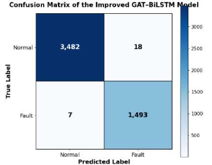
Fig. 2. Confusion Matrix of the Improved GAT–BiLSTM Model.

Table 3. Comparison of the suggested method’s performance with current techniques.

Schemes	Accuracy	Recall	Precision	F1	AUC
DRL + EL [17]	0.985	0.982	0.978	0.980	-
ANN (Smart Ports PdM) [18]	0.987	0.990	0.975	0.980	-
CNN-LSTM [19]	0.961	0.948	0.957	0.952	-
CNN-LSTM [20]	0.964	0.949	0.953	0.951	0.970
ST-GCN	0.989	0.983	0.982	0.982	0.989
GAT-Transformer	0.991	0.985	0.988	0.986	0.993
This work (GAT-BiLSTM)	0.995	0.988	0.995	0.991	0.997

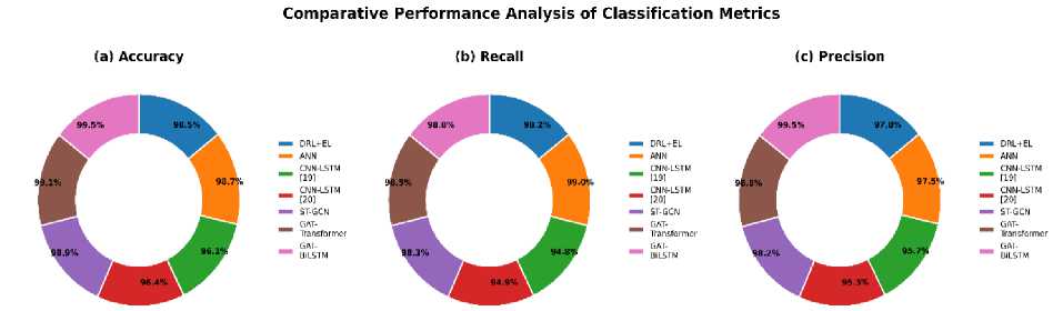
Fig. 3. Comparative Performance Analysis of Classification Metrics.

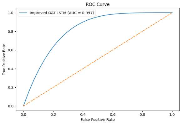
Fig. 4. ROC Curve of the Improved GAT–BiLSTM Model.

As shown in Table 4, this table compares the RUL prediction performance of different deep learning models, showing that the proposed GAT–BiLSTM achieves the lowest error metrics and highest coefficient of determination, indicating improved prognostic accuracy and stability.

• 4.4.    Regression Metrics

The performance of the proposed regression model is quantitatively evaluated using standard error-based and goodness-of-fit metrics. These measures assess how accurately the model predicts continuous target values such as Remaining Useful Life (RUL).

RMSE =

(y t

-Уд2

The Root Mean Square Error (RMSE) measures the square root of the average squared differences between predicted and actual values. It penalizes larger errors more significantly, making it sensitive to outliers.

MAE =

w

1у

NZ-I t=l

I y t - y t I

The Mean Absolute Error (MAE) computes the average absolute difference between predicted and actual values. It provides a straightforward interpretation of prediction error magnitude.

R2 = 1-

Е^у . ^-^)²

Y^Sy t ^{- y)2}

The R2 Score evaluatesR2 how well the model explains the variance in the target variable. A value closer to 1 indicates better model fit and predictive capability.

w

MAPE = ¹⁰⁰ У ^I

N /  , yt t=l

The Mean Absolute Percentage Error (MAPE) measures the average percentage deviation between predicted and actual values. It provides a normalized error metric useful for comparing across different scales. Here, ytrepresents the actual value, ytrepresents the predicted value, ydenotes the mean of actual values, and Nis the total number of samples. As shown in Fig. 5, the scatter plot illustrates strong agreement between predicted and actual RUL values, with points closely aligned along the regression line, indicating high prognostic accuracy and model reliability.

Table 4. Regression Performance Comparison for RUL Estimation.

Model	RMSE	MAE	R²	MAPE
LSTM	9.850	7.420	0.941	0.081
GAT	9.210	6.880	0.948	0.075
CNN-LSTM	8.940	6.630	0.952	0.072
ST-GCN	8.210	6.210	0.958	0.068
GF-GAT	7.980	6.050	0.968	0.065
GAT-BiLSTM	7.820	5.940	0.967	0.061

To evaluate the contribution of each component, an ablation study was conducted by systematically removing key modules. The removal of the dynamic graph module reduced performance due to loss of adaptive relationships. Eliminating cross-attention weakened feature interaction, while removing gated fusion led to suboptimal integration of features. The multi-task learning component significantly improved overall prediction accuracy. These results confirm the importance of each module in the proposed architecture.

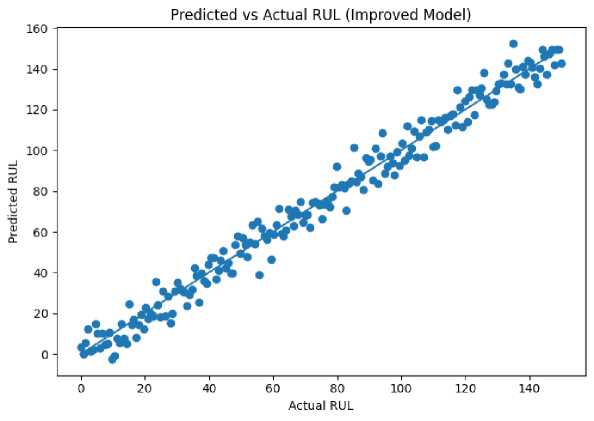
Fig. 5. Predicted versus Actual Remaining Useful Life (RUL) for the Improved Model.

5.    Conclusion

This work presents a dynamic graph-based predictive maintenance framework that integrates Graph Attention Networks (GAT), BiLSTM, cross-attention, and gated fusion to effectively model complex spatio-temporal dependencies in industrial sensor data. The proposed approach demonstrates strong performance in both fault classification and remaining useful life prediction, highlighting its capability to capture evolving relationships among system components. Key findings indicate that dynamic graph construction enhances adaptability, while cross-attention and gated fusion improve feature interaction and representation quality compared to conventional GAT-BiLSTM and static hybrid models. Despite these advantages, the study has certain limitations. The evaluation is primarily based on the SCANIA dataset, which may restrict generalization to other industrial domains. Additionally, the integration of multiple deep learning components increases computational complexity, posing challenges for real-time and edge deployment scenarios. The proposed framework addresses prior limitations by enabling adaptive graph learning, improved temporal modeling, and multi-task optimization within a unified architecture. Future research can focus on validating the model across diverse datasets, reducing computational overhead through model compression techniques, and enhancing robustness to noisy or missing sensor data. Furthermore, exploring lightweight architectures for edge deployment and incorporating self-supervised or transfer learning strategies could further improve scalability and real-world applicability.

All the Declarations and StatementsAuthor Contributions Statement

M. Poonguzhali – Conceptualization, Methodology, Supervision, Project Administration, and Validation. Proposed the research concept, designed the overall framework, supervised the research activities, and reviewed the final manuscript. R. Sujitha – Data Curation, Software, and Investigation. Performed data collection, preprocessing, dataset preparation, and implementation of the proposed framework.

• A. Mahendar – Formal Analysis, Model Training, Validation, and Performance Evaluation. Conducted model training, experimental validation, comparative analysis, and interpretation of the obtained results.

Siva Reddy Sonti – Visualization, Statistical Analysis, and Investigation. Prepared figures, performance visualizations, statistical evaluation, and assisted in experimental analysis.

Malapati Naresh – Writing – Original Draft, Literature Survey, and Documentation. Prepared the initial manuscript draft, conducted the literature review, and documented the technical methodology.

All authors have read and approved the final version of the manuscript.

Conflict of Interest Statement

The authors declare that they have no known competing financial interests or personal relationships that could have appeared to influence the work reported in this paper.

Funding Declaration

This research received no external funding.

Data availability statement

The data used in this study are publicly available. The experiments were conducted using the SCANIA Component X Dataset (Version 2), which is available at:

Accessed on: 11 Jan. 2026

The processed data generated during this study are available from the corresponding author upon reasonable request.

Ethical Declarations

Ethical Approval: Not applicable.

Consent to Participate: Not applicable.

Consent for Publication: Not applicable.

This study does not involve human participants, animals, or identifiable personal data.

Acknowledgments

The authors sincerely thank the Editor and anonymous Reviewers for their valuable comments and constructive suggestions, which significantly improved the quality, clarity, and presentation of this manuscript. The authors also acknowledge the developers of the publicly available SCANIA Component X Dataset for making the dataset accessible to the research community.

Declaration of Generative AI in Scholarly Writing

During the preparation of this manuscript, the authors used OpenAI's ChatGPT to assist with English language improvement, grammar correction, formatting, and manuscript organization. All scientific content, methodology, experimental design, analysis, interpretation of results, and conclusions were independently developed, verified, and approved by the authors. The authors take full responsibility for the accuracy, originality, and integrity of the final published work.

Abbreviations

The following abbreviations are used in this manuscript:

AI - Artificial Intelligence

BiLSTM - Bidirectional Long Short‑Term Memory

CNN - Convolutional Neural Network

DL - Deep Learning

GAT - Graph Attention Network

GNN - Graph Neural Network

IoT - Internet of Things

KNN - k‑Nearest Neighbour

MAE - Mean Absolute Error

MAPE - Mean Absolute Percentage Error

ML - Machine Learning

NLP - Natural Language Processing

RMSE - Root Mean Square Error

ROC - Receiver Operating Characteristic

RUL - Remaining Useful Life

ST‑GCN - Spatial‑Temporal Graph Convolutional Network

TTE - Time‑to‑Event