GraphConvDeep: A Deep Learning Approach for Enhancing Binary Code Similarity Detection using Graph Embeddings

Binary code represents machine-level instructions in a form that computers can execute directly. The goal of similarity detection is to find common patterns or structures between different binary files. Binary code similarity detection involves comparing binary files or executables to identify similarities or differences among them. This process is crucial in various areas, such as cybersecurity, patch detection [1,2], malware analysis [3–5], and software development.

In terms of purpose and applications, BCSD plays a significant role in security by identifying similarities between known and unknown malware to enhance threat detection [6]. BCSD significantly contributes to the security domain by enabling the identification of reused or modified code, which often signals the presence of malware or software vulnerabilities [7– 9]. It plays a crucial role in early threat detection by recognizing shared binary code fragments across different malware variants, thereby uncovering hidden connections between cyber-attacks and facilitating comprehensive threat analysis. BCSD enhances malware detection tools by identifying obfuscated or altered code, making it more difficult for intruders to evade security measures [10].

Additionally, it is valuable in software development to analyze similarities between different versions or builds of software for code reuse or plagiarism detection [10,11]. Furthermore, its application in reverse engineering aids in developing patches and security updates by understanding and addressing vulnerabilities. Various techniques and algorithms are employed for binary code similarity detection, including hash functions that create fixed-size hash values for quick comparisons [12,13], sequence matching using algorithms such as longest common subsequence (LCS), control flow graph (CFG) matching [14], and function-level analysis focusing on comparing functions within binaries. Ongoing developments in the BCSD field include the implementation of machine learning (ML) techniques, which are used for more advanced and adaptive similarity analysis, the exploitation of deep learning techniques on neural networks to extract features and perform similarity comparisons, and the utilization of fuzzy matching methods.

A significant amount of research is actively being pursued, resulting in notable advancements and enhancements across this field . Despite these achievements, challenges continue to remain, such as the code obfuscation techniques used by malicious actors and the efficient handling of large datasets for quick and accurate comparisons. As the landscape of cyber threats evolves, continuous advancements in BCSD algorithms are essential to address emerging challenges and support both cybersecurity and software development processes. As deep learning (DL) continues to excel across various domains, such as recommendation systems, anomaly detection, and healthcare, more experts have innovated techniques to identify similarity via neural networks. The novelty of the approach are as follows:

• •    The approach creates embeddings for binary functions via graph convolutional networks (GCNs), which capture complex relationships, handle the variability present in binary code and adapt to different code structures.

• •    During model training, a comprehensive cross-platform dataset comprising 129,364 binary files is constructed by compiling the open-source Linux packages across various optimization levels. Compared with state-of-the-art techniques, such as Genius [15], Gemini [16], and DeepDualSD [17], the experimental results demonstrate the good performance of the proposed approach.

• •    To search for vulnerabilities, a dataset was created that included firmware images and vulnerable functions from the CVE database [18]. By employing similarity detection technique to compare firmware images and known vulnerabilities, proposed approach effectively identified vulnerable firmware images. The experimental results demonstrate that the proposed method has the best accuracy, 95%, in identifying similarities among code fragments, thus demonstrating its effectiveness in cross-platform BCSD.

2.    Literature Survey

The subsequent sections of the article are outlined as follows: A literature review of the existing BCSD methods is presented in Section II. Section III explains the proposed DL-based solution. Section IV offers a comparative analysis between the proposed method and other established BCSD techniques. The conclusions of this work are provided in Section V.

In this section, existing methods such as graph matching, deep learning-based methods for BCSD are discussed. Over the past two decades, numerous methodologies have been introduced by researchers to analyze binary code similarity. These approaches have been extensively utilized to address critical issues, including bug identification, malware detection, patch analysis and malware analysis. However, challenges persist within this domain, such as code obfuscation, variability in programming styles, compiler optimizations, and platform-specific characteristics, which can introduce noise and variability in binary code, dynamic behaviors exhibited by software at runtime and cross-platform compatibility. Because of persistent challenges, conducting a comprehensive literature survey in this field is imperative.

Genius [15] proposed a codebook generation approach to solve the scalability challenge present in the bug search approach across different platforms. Xu et al. [16] proposed method, which uses neural networks (NNs) to compute embeddings for each binary and is designed to address the cross-platform BCSD problem. The model outperforms the control flow graph approaches in terms of accuracy and efficiency, demonstrating superior performance in similarity detection tasks. The model leverages a Siamese network for training the embedding network, allowing for the generation of embeddings that capture persistent features of binary functions across different compilers and architectures. The model's adaptability is demonstrated through its ability to be quickly retrained for specific tasks and achieve high accuracy in identifying vulnerable firmware images. Furthermore, the visualization of the embeddings demonstrates the model's effectiveness in preserving information about the source functions across different target architectures, compilers, and optimization levels. The work presented in [17] outlines a dual-attribute embedding approach that combines the semantic and structural attributes of binary code to improve BCSD performance.

Jinxue PENG et al. [19] introduced fast cross-platform BCSD to address the issues of high convolutional computation and structural information loss faced in techniques designed using CFGs and GCNs. The approach employs natural language processing (NLP) for basic block embedding, and for function representation, inductive GNN GraphSAGE (GAE) is used.

The CrossDeep [20] approach discusses cross version binary similarity model-based CNN and encoding methods. The proposed work combines raw byte analysis with CNN to enhance accuracy of similarity detection. The SimInspector [21] method proposes advanced techniques such as the neural machine translation (NMT) model and the graph embedding model. These models extract semantics of binary code, leading to improved accuracy in similarity detection. This can be achieved by training an NMT model [22] and a graph embedding model to automatically extract binary code semantics, which are represented as numerical vectors. This work evaluates the effects of different hyperparameters on model accuracy, providing insights into the optimal settings for achieving the highest performance.

A novel solution for binary code similarity comparison was discussed in [23], which addresses the challenges posed by compilation diversity and code obfuscation. A multiview approach that combines structural, semantic, and syntactic features of functions is extracted for embedding. The technique achieves higher recall than the baseline in vulnerability function search does, highlighting its effectiveness in real-world vulnerability detection. Yuede Ji et al. [24] explained how high accuracy and code coverage challenges are addressed. The efficiency is achieved through two different steps, namely, binary source canonicalization and code similarity calculation. The system uses an Attributed Control Flow Graph (ACFG) to collect the raw features from binary code and employs a GNN model to compute representative embeddings for each attributed graph. Additionally, the work also includes a graph triplet-loss network (GTN) for ranking the similarity of binary functions and supervising the learning process.

A deep learning (DL) approach [25] aims to address limitations such as dependency on engineered syntactic features for similarity comparison. The proposed technique, i.e., BinDeep, uses a recurrent neural network (RNN) DL algorithm to recognize the types of target functions. To measure the similarity between two entities, a Siamese neural network is employed, leveraging a fusion of convolutional neural networks (CNNs) and long short-term memory (LSTM). The model uses instruction embedding with vectorizing the extracted instructions. Yang, S. et al. [26] proposed the semantic resemblance of functions across different architectures via the abstract syntax tree (AST) encoding method. The Tree-LSTM network is used to capture function semantic representation. ASTERIA successfully detects vulnerable functions in Internet of Things (IoT) firmware images, emphasizing its practical application in vulnerability search. The method uses the Siamese architecture to combine two similar Tree-LSTM models for AST similarity detection.

The binary search engine described in [27] matches semantically equivalent and similar functions across different architectures, operating systems, and compilers. A selective inlining approach will learn the whole function semantics, and three filtering processes are narrowed down to match the candidate target functions. The selective inlining technique greatly enhances the overall matching accuracy, particularly for ARM binaries. Problems such as dynamic analysis difficulties for firmware, handling a single architecture and using semantic similarity for analyzing large code bases are addressed in discovRE [28]. The technique discovRE identified POODLE and Heartbleed vulnerabilities of Android images in approximately 80 ms.

Existing solutions primarily rely on individual features, which limits their ability to capture the complex relationships within program behavior, resulting in lower accuracy. In contrast, the Attributed Control Flow Graph (ACFG) integrates both structural and syntactic features information, providing a more comprehensive representation. The choice of the Attributed Control Flow Graph (ACFG) feature in GCN, helps to improve accuracy in similarity detection. For binary structural features, GCNs are an optimal choice due to their ability to effectively capture and propagate structural dependencies within graph-based data. The choice of the specific GCN model was based on its effectiveness in capturing structural relationships within graph-structured data. GCNs have been widely used for node classification and graphbased learning tasks due to their ability to aggregate information from neighboring nodes. Hence, GraphConvDeep, a Graph CNN, is proposed.

3.    Proposed Approach

This section outlines the main ideas of the proposed approach. The overview of proposed model is provided in subsection 3.1. The feature extraction from the binaries is explained in subsection 3.2. Subsection 3.3 presents the computation of ACFG embedding. Finally, the use of the Siamese architecture in the proposed model is explained in subsection 3.4.

• 3.1.    Solution Overview

• 3.2.    Feature Extraction

Figure 1 shows an overview of the proposed technique GraphConvDeep. The block level and interblock parameters are obtained from the source and target binaries. This preprocessing stage, which extracts features, is called feature extraction. The extracted features are converted into ACFG. The ACFG encompasses block-level attributes, interblock attributes for every node, the total node count in the graph, source filename, and edge details within the graph. The ACFG is an input to the GraphConvDeep Embedding Model, which generates graph embedding, i.e., a high-dimensional vector based on the CFG of each binary function. The model computes the vector by passing through four steps. The steps include node degree computation, neighborhood aggregation, linear transformation of node features and a message passing mechanism. In the first step, the degrees of every node in a graph are computed by adding self-loops to the graph, providing valuable information about the node's connectivity within the graph structure. The primary reason for adding self-loops in GCNs is to ensure that each node's own feature representation is also considered during the aggregation step. In the second step, every node representation is updated on the basis of information from neighboring nodes in a graph. Neighborhood aggregation allows nodes to gather and integrate information from their local environment, resulting in refined and context-aware representations that are crucial for various tasks, such as linear transformation and message passing mechanisms. The input feature matrix undergoes a linear transformation during the third step, which is the forward pass of a GCN layer. A linear transformation stage aims to project the feature vectors into a new space, potentially of higher dimensionality. The transformation enables the model to acquire more complex representations of the input data. The final step is the message passing mechanism in GCNs, where nodes exchange and gather information to revise their representations by utilizing the graph structure and input features. At the GCN output later, the final graph embeddings are computed based on the aggregated and transformed feature vectors obtained from the previous stages. The final graph embedding from the output layer is passed to the Siamese architecture for comparison. The Siamese architecture [29] takes two embeddings of different binaries and generates a similarity score via a similarity measure. Specifically, the proposed model mainly consists of three stages: feature extraction, ACFG embedding and similarity computing, which will be discussed in the following sections.

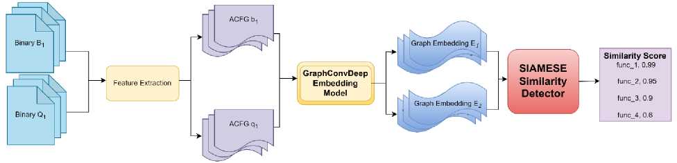
Fig.1. Overview of the proposed approach, GraphConvDeep

In binary code similarity detection, both block-level parameters and interblock parameters [15] are essential for capturing the structural and behavioral characteristics of the binary code. Table 1 lists the basic block parameters, which include both block level and interblock parameters. The block level and interblock parameters are as follows: Block-level parameters: These attributes refer to characteristics or properties associated with a block of code. Curly braces {} in languages such as C, C++, or Java typically contain a group of statements for creating a block of code.

• •    String literals: String literals are fixed values of characters (text) that do not change during program execution. For example, "Hello, World!" is a string constant.

• •    Numeric literals: Numeric literals are fixed values of numbers that do not change during program execution. For example, 42 is a numeric constant.

• •    No. of Transfer Instructions: Transfer instructions refer to statements that control the flow of the program, such as conditionals (if, if-else, switch) and loops (while do-while for). The transfer instructions count can provide insights into the program's control flow complexity.

• •    No. of Calls: This attribute typically refers to the number of functions or method calls within a block of code. It indicates how often other pieces of code are invoked.

• •    No. of Instructions: This attribute represents the total count of instructions within a block. It provides a measure of the size or complexity of the code.

• •    No. of Arithmetic Instructions: Arithmetic instructions refer to basic mathematical operations such as summation, subtraction, product calculation, and division. The number of arithmetic instructions helps to evaluate the computational complexity of a block of code.

Interblock attributes: These attributes involve relationships or characteristics between different blocks of code.

• •    No. of Offspring: In the context of code analysis, the offspring count usually refers to the number of blocks that are directly executed as an output of the current block. It provides insight into how control flow is distributed.

• 3.3.    ACFG Embedding

Figure 2 depicts the partial control flow graph and ACFG of the Heartbleed vulnerability function present in the OpenSSL Linux package. The seven features extracted are shown in the attributed control flow graph of vulnerability function.

Table 1. Basic block parameters

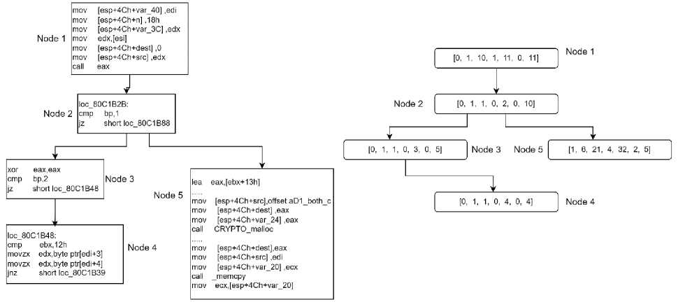
Fig.2. Partial CFG of the dtls1_process_heartbeat (heartbleed vulnerability) function and its ACFG

Block-level parameters	Interblock parameters
String literals	Offspring Count
Numeric literals
Transfer Instructions Count
Calls Count
Instructions Count
Arithmetic operations Count

The features extracted are used to compute embedding of each node in a graph and then one final graph embedding. The graph embedding generation process aims to generate an embedding vector for the input graph. It starts by processing each vertex in the graph, calculating node degrees and normalization factors, applying a linear transformation to the associated features, message propagation and final embedding computation. Algorithm 1 represents the detailed process of embedding computation. The input is an Attributed Control Flow Graph (ACFG) represented as G = (V, E, f) where V is the set of vertices (nodes), E is the set of edges (connections between nodes) and f v is the feature vector of each node v. The algorithm iterates over L convolution layers. For each node v in the graph, the following computations occur:

Algorithm 1: Graph Embedding Generation

Input :              ACFG G = (V, E, f)

Set of Vertices: V, Set of Edges: E,

Set of basic-block features of each vertex in the graph: f

Hyperparameters: Learnable Weight Matrix: W

Output :            Final Graph Embedding: ɸ(G)

1.	for t =1 to No. of Convolution Layers (L)
2.	for each node v € V do
3.	d i = Z jeX(i) A;	(Compute Node Degree)
4.	A ■• = AiJ 'I    Jd l d J H« +1) = (a .Hw .W(i))	(Compute Normalization Factor using node degrees)
5.		(Linear Transformation of Node Features f)
6.	mv = Еиел-адЛ .4.H(1+1)	(Message Passing)
7.	H ' = a(mv)	(Apply Activation Function RELU (a))
8.	end for
9.	end for
10.	ф(G) = Aggregate (H ' )	(Aggregation of all the node embeddings )
11.	return ɸ(G)

• A.    Node Degree Calculation

For each node V t in the graph, calculate its degree d t :

di — ^jeN(t) Atj where Atj is the adjacency matrix element indicating the connection between nodes i and j,^(^) denotes the set of neighboring nodes of vt. This stage helps in understanding the structural role of each node, distinguishing between highly connected nodes (hubs) and isolated nodes.

• B.    Normalization Factors

Calculate the normalization factor for each node V t using the degrees of the nodes

л

A

where A_t j is the normalized adjacency matrix. Normalization factors prevent overemphasis on high-degree nodes, reducing bias in message aggregation, improves numerical stability and convergence during training.

• C.    Linear Transformation

Apply a linear transformation to the features of each node. Let X 6 K ^^xf represent the input feature matrix, where N is the no. of nodes and F is the no. of features per node. The linear transformation is defined as:

H < ⁱ⁺¹ ) — (A.h^(,).w^(,))                                               (3)

where H⁽¹⁺¹⁾ is the updated feature for node v _t at the next layer I + 1. H® is the hidden feature matrix at layer I ,with H⁽⁰⁾ — X, W⁽ⁱ⁾ 6 R^FxF ' is the trainable weight matrix at layer I, a(-) is a non-linear activation function and A is the normalized adjacency matrix from the previous step.

• D.    Message Propagation

The process of message passing [30] and feature updating in a GCN begins after a linear transformation applied to each node's features. This transformation prepares the features for aggregation. With each layer, nodes aggregate information from their immediate neighbors, and by stacking layers, nodes can capture information from increasingly larger neighborhoods in the graph. The key idea is that every node collects information from its neighbors, and the node representations are updated through a neural network layer.

At each iteration of message passing, a hidden embedding is updated for every node based on information collected from its graph neighborhood. Figure 3 depicts the message passing mechanism, where each node in the GCN calculates its embedding by gathering information from its neighbors.

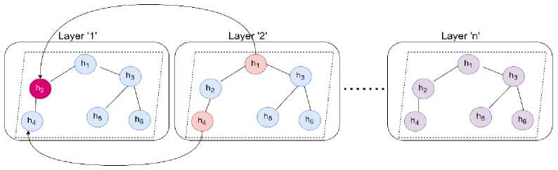
Fig.3. Neural message passing mechanism in the GCN

• E.    Embedding Computation

The rectified linear unit (ReLU) activation function is performed elementwise at the output of the message passing operation. This stage introduces nonlinearity into the network and helps in dimensionality reduction, making the computation more efficient.

H’ = а(т)

The final embedding vector ф(б) for the entire graph can be obtained by aggregating the node embeddings,

ф(6) = Aggregrate(H’)

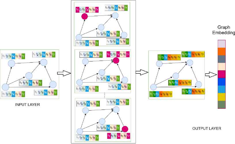
where H ’ is the output feature matrix from the final layer L , and the average is the aggregation function. Figure 4 illustrates the graph embedding computation in GCN. The process begins with the initial node features, followed by message passing where each node aggregates information from its neighbors. The process is repeated for the ‘ L ’ number of convolution layers. Finally, an aggregation function processes the final layer's output, resulting in an updated embedding vector of the input graph. The updated embedding vector can be useful for finding matching functions.

HIDDEN LAYER

Fig.4. Graph convolutional network (GCN) architecture utilized for generating graph embedding

• 3.4.    Siamese Similarity Detection

The Siamese neural network is a deep learning architecture designed for similarity learning, where two identical subnetworks process different inputs while sharing the same parameters. Each subnetwork extracts feature representations from its respective input, ensuring that the learned features remain consistent across both networks. Siamese architecture [29] refers to a design pattern or architectural style in which two identical or similar structures are conjoined or connected in some way. The Siamese architecture in BCSD refers to the use of neural network architectures inspired by Siamese networks to detect similarities or dissimilarities between binary code samples. Siamese networks are neural network architectures characterized by two identical subnetworks known as twins, which share identical parameters and are trained simultaneously on pairs of input data. This architecture is particularly effective in binary similarity detection, where structural patterns in binaries can be analyzed and compared to identify relationships, making it useful for tasks like malware detection and software lineage analysis. The Siamese architecture is the best fit for binary code similarity detection because it effectively learns and compares structural and semantic patterns between binary representations. Unlike traditional classification models that assign discrete labels, the Siamese network focuses on measuring the similarity between two inputs, making it ideal for comparing binary files without requiring an extensive labeled dataset.

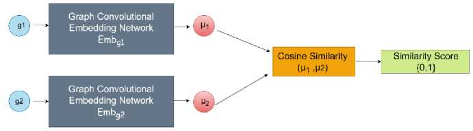
Fig.5. Siamese architecture

In the GraphConvDeep model, the Siamese layer takes two embeddings from different binaries and computes the similarity score based on the similarity metrics, cosine similarity and jaccard similarity coefficient metric. The Siamese architecture employed in the proposed method using cosine similarity is depicted in Figure 5. The cosine similarity among two binary code samples is calculated by the dot product of their normalized feature vectors and dividing the result by the product of their Euclidean norms. Mathematically, it can be expressed in Eq. 7.

A-B

Cosine Similarity (A,B) = — where:

• •    A and B are the normalized binary feature vectors representing two binary code samples.

• •    represents the dot product operation.

• •    |A| and |B| denote the Euclidean norms of vectors A and B , respectively.

The Jaccard similarity coefficient is a measure of similarity between two vectors. It is defined as the size of the intersection divided by the size of the union of the two vectors. Mathematically, it can be expressed as:

Jaccard Coefficient(A,B) = |AAB1

where :

• •   |Л A B| is the no. of elements in the intersection of vectors A and B,

• •   |A U B | is the no. of elements in the union of vectors A and B

4.    Evaluation

• 4.1.    Experimental Setups

  Using the PyTorch backend library and the Keras [31] platform, the proposed method was developed in Python. The experiments were conducted on an HP Z4 G5 Workstation - 1x Intel Xeon Octa-core w3-2435 (8 Core) server running the Windows 10 operating system with a processor speed of 3.10 GHz, 512 GB solid-state drive (SSD) secondary memory, 16 GB SDRAM DDR5 internal memory and NVIDIA T1000 4 GB graphics. Binaries are disassembled using the Binary Ninja open source tool [32]. The plugin in the IDA Pro tool is utilized to extract the ACFG from binary files [33].

• 4.2.    Dataset

This section focuses on the analysis of the experimental results obtained by the proposed model and the comparative analysis with the cutting-edge methods.

The proposed model is evaluated on 3 datasets. Dataset 1 is derived from OpenSSL across multiple compiler optimizations and CPU architectures, ensuring a balanced set of function pairs for supervised learning in binary similarity analysis. Dataset 2 consists of function graphs extracted from diverse firmware images of multiple vendors, categorized by size to evaluate efficiency and reduce bias in analysis. Dataset 3 includes vulnerable functions from real-world security exploits, compiled under different optimization settings to study patterns across software from various vendors.

Dataset 1: The dataset was prepared by selecting a popular Linux package, OpenSSL (v3.0.0 to v3.3) [34]. OpenSSL is a widely used open-source cryptographic library. OpenSSL is used in binary similarity analysis because many binaries include its cryptographic functions, making it useful for detecting code reuse, software lineage, and security vulnerabilities. OpenSSL functions have well-known signatures, making it easier to compare binaries based on functionlevel similarity. Following the acquisition of the package source code, each program is compiled using GCC and Clang compiler with four optimization stages (O0, O1, O2, O3) and three CPU architectures (ARM, x86 and MIPS). The matched and unmatched function pair counts used in training and testing are reasonably balanced to aid in supervised learning. Functions are randomly selected from several binaries with distinct function names to obtain the negative training examples. Positive and negative samples are extracted and stored in different files with similar and dissimilar labels, respectively. For the experimental observations, 129364 samples were considered. This selection ensures a fair comparison, as other baseline approaches have also utilized same Linux package in their evaluations. The ACFG counts across the different platforms used for training and testing are displayed in Table 2. The sample consists of 38,794 X86, 38,610 ARM and 51,960 MIPS (Microprocessor without Interlocked Pipelined Stages) binaries. To assess the method's binary performance, three distinct subsets of the entire dataset are used for testing and training. For ablation studies, Dataset 1, which comprises 129364 functions, is further subdivided into three subsets of across different compilers, optimization levels and architectures. The complete dataset is partitioned into two subsets, with 30% allocated for testing and 70% allocated for training.

Table 2. ACFG Counts in the Dataset 1

	X86	ARM	MIPS	TOTAL
Training	27155	27027	36372	90554
Testing	11639	11583	15588	38810
TOTAL	38794	38610	51960	129364

Dataset 2: A dataset containing ACFGs of varying sizes, based on the vertex count in each graph, is constructed to assess efficiency. Specifically, ten firmware images are chosen at random from Dataset II used in [15]. With sizes varying from 1 to 1,306 vertices, 54,200 ACFGs are derived from these 10 firmware images. The firmware images are from Dlink, TPlink, Netgear, Cisco, vendors. This diversification helps mitigate bias and ensures evaluation across a broader range of binaries. To ensure that every ACFG in a set is the same size, these ACFGs are arranged into sets according to size. Eighteen ACFGs are chosen at random from each set that has more than 18, with the remaining ACFGs being eliminated. For the dataset II, 2,785 ACFGs are ultimately obtained.

Dataset 3 : The dataset includes 121 vulnerable functions of four different vendors obtained from the CVE database [18]. The functions are compiled using GCC and Clang compiler with four optimization stages (O0, O1, O2, O3). The dataset is designed to analyze vulnerable function patterns from real-world exploits. Binaries are extracted from documented security vulnerabilities in widely used software. The functions were selected based on severity, exploitability, and frequency of occurrence, which could introduce biases. Even though Dataset 1 was prepared from OpenSSL package, Dataset 2 from specific vendors, and Dataset 3 from a vulnerability database, biases exist in terms of dataset size and vendor representation. However, each dataset was designed separately to support different types of analysis, ensuring targeted evaluations rather than direct comparisons.

• 4.3.    Evaluation Metrics

The performance metrics like precision rate (PR), accuracy (Acc), F1 score (F1), average running time (ART) and recall rate (RR) are used to analyze the performance of the proposed model. Metrics are well-suited for binary similarity detection because they effectively quantify the model's ability to distinguish between similar and dissimilar binary files. These metrics are defined as follows:

• •    Acc measures the overall correctness of the model but can be misleading in imbalanced datasets. Since binary similarity detection may involve imbalanced pairs (e.g., more dissimilar pairs than similar ones), accuracy alone is insufficient.

• •    RR is critical in this context as it indicates the proportion of actual similar binaries that are correctly identified. A high recall ensures that most similar binaries are detected, which is essential for malware analysis, vulnerability detection, and software lineage tracking.

• •    PR evaluates how many of the detected similar binaries are truly similar. A high precision prevents false positives, ensuring that detected similar binaries are genuinely related.

• •    F1 balances precision and recall, making it a more reliable metric in scenarios where both false positives and false negatives are costly. Since binary similarity detection involves trade-offs between missing similar binaries and wrongly identifying unrelated binaries as similar, the F1-score provides a comprehensive evaluation.

• •    The total running time (TRT) and the ART are employed to evaluate efficiency. The TRT is the sum of running time per round, and the ART is defined in Eq. 13, where γ is the training round number.

  Acc =

  
  

  TP+TN

  TP+TN+FP+FN

  
  

  PR =

  
  

  TP

  TP+FP

  
  

  RR =

  
  

  TP

  TP+FN

  
  

  F1 = 2 *

  
  

  Precision*Recall

  Precision+Recall

  
  

  ART = — v

  
  
  
  

• 4.4.    Performance Analysis

  Dataset 1 is considered for the experiment. 129,364 ACFGs are present in the dataset, 90,554 ACFG’s are used to train the model and 38,810 ACFG’s are used for testing. The values in Table 3 show that the best accuracy score is 0.9592, and the recall rate is 0.9448 after 100 epochs. As the no. of epochs increases, the best accuracy and recall rate are observed in the model. The F1_score is 0.9390, and the precision rate is 0.9334, which means that a higher F1 score and precision rate indicate that the model makes more accurate positive predictions while minimizing false positives, which generally signifies better performance in binary classification tasks. Figure 6 shows the different performance metric results of the proposed approach method.

These metrics are essential for assessing the performance of classification techniques and provide insights into different aspects of their effectiveness, such as overall accuracy, ability to correctly classify positive instances, and ability to identify all relevant instances. Table 3 summarizes the PR, Acc, F1 and RR values achieved by GraphConvDeep on the testing dataset. The metric values are tabulated over different numbers of epochs.

Table 3. Performance metric results achieved by proposed approach on the testing dataset 1

Epoch	Acc	RR	PR	F1
10	0.9272	0.9109	0.9292	0.9199
20	0.9216	0.9263	0.9345	0.9303
30	0.9263	0.9295	0.9392	0.9343
40	0.9325	0.9234	0.9292	0.9262
50	0.9358	0.9316	0.9307	0.9311
60	0.9443	0.9263	0.9392	0.9327
70	0.9482	0.9309	0.9308	0.9308
80	0.9443	0.9463	0.9492	0.9477
90	0.9591	0.9339	0.9434	0.9386
100	0.9592	0.9448	0.9333	0.9390

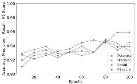
Fig.6. Performance metric results of the proposed method

Accuracy in Different Function size: The statistical analysis is conducted by taking function size (number of nodes in ACFG) present in Dataset 1 across a total number of target functions with similarity detection accuracy. In Table 4, the first column delineates the range of function sizes, and the second column enumerates the no. of functions falling within each size range. The function sizes span from 5-900, with the majority being less than 50. In the third column, the accuracy of similarity detection corresponding to functions of varying sizes is presented. The accuracy falls within the range of 0.9397-0.9592, indicating notably consistent and reasonably accurate detection across the spectrum of function sizes. Notably, there was no discernible trend suggesting diminishing accuracy with increasing function size.

Table 4. Function size distribution in the dataset and detection accuracy achieved in proposed approach

Function Size	Function #	Detection Accuracy
{5,50}	51446	0.9592
{50,100}	3249	0.9554
{100,200}	1078	0.9499
{200,300}	224	0.9588
{300,400}	94	0.9473
{400,500}	91	0.9397
{500,900}	81	0.9492

Evaluation of the hidden units in proposed approach: The no. of hidden units in neural networks directly influences how well they can recognize and interpret complex patterns in data. Increasing the no. of hidden units can enhance the network's capability to capture intricate relationships within the data, potentially leading to improved performance metrics such as accuracy. Selecting an appropriate number of hidden units is crucial for optimizing the balance between model complexity and generalization ability, ultimately impacting the neural network's performance. Our experiments investigating the impact of varying the no. of hidden units in GNNs reveal significant effects on the results. Ranging from 1 to 25 different hidden units on the GraphConvDeep approach, the findings are illustrated in Figure 7(a). The number of hidden units in neural networks can also affect their running time. Generally, increasing the no. of hidden units typically leads to longer training and inference times because of the greater computational complexity involved in processing more parameters and performing more calculations. This increased computational demand arises from the need to propagate information through additional layers and units, resulting in longer processing times. Figure 7(b) indicates that the ART of the proposed method after 20 epochs remains stable. The experimental results indicate that there is a consistent trend as the hidden units increases. Acc, RR, PR and F1 generally improve, whereas ART remains relatively stable in the range of 29-36. After 20 epochs, the four performance metrics listed in Table 5 remain stable. Based on thorough experimental analysis, it is evident that selecting 20 as the number of hidden units represents an optimal choice.

Table 5. Performance metric results achieved by proposed approach for different hidden units

Hidden Units	Acc	PR	RR	F1	ART(s)
1	0.9240	0.9430	0.9310	0.93696	29
5	0.9359	0.9490	0.9390	0.94397	31
10	0.9351	0.9459	0.9490	0.94745	35
15	0.9321	0.9377	0.9469	0.94228	28
20	0.9591	0.9494	0.9331	0.94118	28
21	0.9592	0.9594	0.9441	0.95169	33
22	0.9593	0.9454	0.9433	0.94435	34
23	0.9584	0.9424	0.9453	0.94385	35
24	0.9583	0.9434	0.9633	0.95325	36

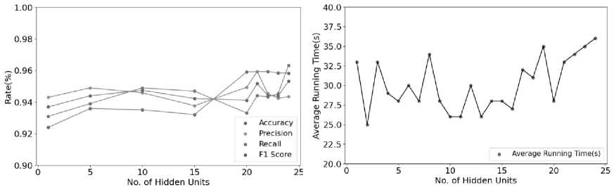
Fig.7. (a) Hidden unit vs performance metric (b) Hidden unit vs ART

• 4.5.    Hyperparameters

This section evaluates the efficacy of hyperparameters in the proposed approach by analyzing the influence of training epochs and loss [35].

• •    Number of Graph Convolutional Layers : Graph Convolutional Networks likely involves multiple layers of graph convolutional operations. The depth of these layers can impact the model's capacity to capture complex relationships in the data. The number of layers created in the proposed approach is 21. Based on the observed experimental results, the best performance was achieved with 21 layers in the proposed approach.

• •    Hidden Dimensionality: The number of hidden layer representations in the graph convolutional layers. This parameter determines the dimensionality of the embedding space and can significantly affect model performance. The no. of hidden layers used in the proposed approach is 20.

• •    Activation Functions: The selection of activation functions used in the neural network layers includes ReLU, leaky ReLU, and sigmoid. The ReLU is used in the hidden layers of the GCN because it is simple and computationally efficient and avoids the vanishing gradient problem. Sigmoid functions are employed in the output layer of binary classification problems where the objective is to produce probabilities. The sigmoid function produces outputs in the range (0, 1), which can be interpreted as probabilities.

• •    Training Epochs: The model underwent training for 200 epochs, with evaluations conducted over the test set every 10 epochs to measure both the AUC and loss. The findings are depicted in Figure 8(a) and Figure 8(b). Figure 8(b) shows a gradual improvement in the AUC value, which stabilizes around epoch 35, whereas the loss value rapidly decreases and remains relatively stable after the same epoch. From the analysis shown in Figure 8(a) and Figure 8(b), it is evident that the model can be trained faster to obtain improved efficiency.

• 4.6.    Comparative Analysis

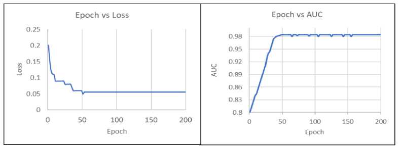
Fig.8. (a) Loss vs. epochs (b) AUC vs. epochs

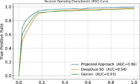
The binaries of X86, ARM, and MIPS platforms present in Dataset I are selected. The proposed method is evaluated on ACFG pairs from the dataset. [16] and [17] are used as the standard baseline methods for comparison, and their accuracies are assessed on the same testing dataset. The receiver operating characteristic (ROC) curves of the three methods are displayed in Figure 9. The proposed approach ROC is shown to be closer to the top and left borders, obtaining a substantial area under the curve (AUC) value (average 96% across platforms), indicating that the proposed technique is more accurate. Table 6 lists the different AUC values obtained via the three different approaches. In the ARM vs. x86 comparison, the result of proposed approach is 5% higher than that of DeepDual-SD [17] and 6.1% higher than that of Gemini [16]. The result of GraphConvDeep is 4% higher than that of Gemini in the case of MIPS vs ARM. DeepDual-SD and proposed approach are almost equal in the cases of MIPS vs ARM and x86 vs MIPS. It is evident from the results that proposed approach achieves better performance than the other two approaches do in the case of the x86 vs ARM comparison.

Table 6. Performance comparison of the proposed approach with other cross platform methods

Platforms	Gemini [16]	DeepDual-SD [17]	Proposed Approach
ARM vs x86	0.93	0.94	0.98
MIPS vs ARM	0.92	0.93	0.95
x86 vs MIPS	0.92	0.94	0.94
Average	0.93	0.94	0.96

False Positive Rate

Fig.9. ROC curves of the proposed approach using different models

Efficiency of embedding models: The efficiency of LSTM+GAE [19], LSTM+GAT [19], Structure2Vec DNN [36] and proposed approach for embedding generation is evaluated using Dataset II . The deployment of an approach hinges significantly on its inference time. Therefore, the total runtime and test time of the four methods are recorded in Table 7. The dimension is identified by the embedding scheme used. The TRT is scaled according to the dataset size. The experimental results indicate a positive correlation between the input dimension and the inference time when identical GNN models are employed. The running and test time of LSTM+GAE [19] are 3227 and 75.5 s, respectively, when the embedding dimension size is 100. The Structure2Vec DNN method with a dimension size of 50 has a running time of 7373 and a test time of 345.6 seconds. The proposed method has a running time of 2495 s and a test time of 32 s with a dimension size of 75. The results suggests that the proposed model takes less time than the other three approaches do.

The first 25 epochs running times of the three different models are depicted in Figure 10. The time overhead is lower in the GraphConvDeep technique than in the other two approaches. The experimental results shows that baseline approaches are slow, while the proposed method demonstrates superior speed and flexibility.

Table 7. Time analysis comparison of the proposed approach with existing embedding models

Scheme	Dimension	Running time (s)	Test time (s)
LSTM+GAE[19]	100	3227	75.5
LSTM+GAT [19]	100	3886	56.8
Structure2Vec DNN[36]	50	7373	345.6
Proposed Approach	75	2495	32.1

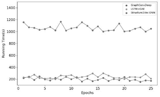
Fig.10. Running times of proposed approach and other embedding models for the first 25 epochs

Vulnerability Detection Analysis: The technique is evaluated on firmware images encountered in the real world. The two vulnerabilities were selected from the Dataset III. The two vulnerabilities used in the Genius [15] and Gemini [1 6] techniques are CVE-2015--1791 and CVE-2014--3508. In the case of CVE-2015--1791, Genius has 28% precision in detecting vulnerable firmware images, which are exclusively from D-Link and Belkin. The Gemini technique identified 42 true positives with 85% precision from four different vendors, such as Tomato by Shibby, DD-wrt, ZyXEL and D-Link, which were included in the top 50 results. The proposed method is able to detect 45 true positives from all vendors considered for evaluation. This was possible because of the task-specific retraining approach using a GCN. In the case of CVE-2015-3508 vulnerability, the control flow graph does not change much, so it is difficult to find. Among the top 50 results, Genius identified 24 firmware images as vulnerable, achieving a precision rate of 48%. Gemini detected vulnerabilities in 41 out of the top 50 firmware images, achieving a precision rate of 82%. The proposed technique was successful in detecting 46 firmware images from the top 50 results with a precision of 95%. The precision rates and numbers of vulnerable firmware images detected in the top 50 results of Genius [15], Gemini [16] and the proposed techniques are shown in Table 8. By employing the proposed technique, organizations can effectively manage and mitigate security risks associated with CVE-listed vulnerabilities.

In IoT security, where firmware is often closed source and reverse engineering is complex, proposed similarity detection model significantly enhances vulnerability detection efficiency. Proposed model allows vulnerabilities found in one architecture (e.g., ARM) to be efficiently mapped to others (e.g., MIPS, x86), reducing the need for redundant manual analysis. Cross-platform similarity detection solution enhances vulnerability detection in IoT firmware by enabling seamless identification of security flaws across different architectures, compilers, and optimizations. It helps in proactive risk assessment, cross-platform security consistency, and automated identification of both known and structurally similar vulnerabilities.

Table 8. Comparison of precision rate and vulnerable firmware identifications of the proposed approach with other cross-platform methods

Technique	CVE Vulnerable Name	Precision	No. of vulnerable firmware images detected out of Top 50
Genius [15]	CVE-2015-1791	28%	14
	CVE-2014-3508	48%	24
Gemini [16]	CVE-2015-1791	84%	42
	CVE-2014-3508	82%	41
Proposed Method	CVE-2015-1791	94%	45
	CVE-2014-3508	95%	46

• 4.7.    Ablation Study

5.    Conclusions

Table 9. The Ablation models of proposed approach

	Features
Model	Cross Compiler	Cross Optimization	Cross Architectures
Base	✓	✓	✓
A1	✓		✓
A2		✓	✓
A3	✓	✓
A4			✓
A5		✓
A6	✓

Table 9 outlines the ablation models of the proposed approach, focusing on the inclusion or exclusion of three key features: cross compiler, cross Optimization, and cross architectures. The Base model incorporates all three features, representing the full version of the proposed approach. Models A1 through A6 systematically exclude one or more features to evaluate their impact on performance. A1 excludes cross Optimization, A2 excludes cross compiler, and A3 excludes cross architectures. The remaining models (A4, A5, and A6) include only one feature, cross architecture, cross optimization and cross compiler respectively, allowing for a deeper understanding of each component's individual contribution.

Table 10. Ablation study of proposed approach on dataset 1 and dataset 2

	Dataset 1				Dataset 2
Model	Accuracy	Precision	Recall@1	F1 Score	Accuracy	Precision	Recall@1	F1 Score
Base	0.95	0.94	0.93	0.93	0.96	0.94	0.95	0.94
A1	0.93	0.93	0.92	0.92	0.91	0.92	0.93	0.92
A2	0.94	0.93	0.91	0.91	0.92	0.93	0.91	0.91
A3	0.91	0.89	0.91	0.89	0.83	0.84	0.86	0.84
A4	0.92	0.91	0.93	0.91	0.78	0.88	0.79	0.83
A5	0.89	0.86	0.89	0.87	0.89	0.86	0.89	0.87
A6	0.87	0.78	0.79	0.78	0.81	0.73	0.78	0.75

Table 10 presents the results of an ablation study, comparing the performance of various models on Dataset 1 and Dataset 2 across four metrics. The Base model, which includes all three features (Cross Compiler, Cross Optimization, and Cross Architectures), achieves the highest performance on both datasets, with Dataset 2 showing slightly better accuracy (0.96) and recall (0.95). In contrast, Model A6, which only includes Cross Compiler, consistently exhibits the lowest performance across all metrics for both datasets, highlighting the insufficiency of relying solely on a single feature. The high performance of the Base model suggests that the combination of all three features is crucial for optimal results, as they likely complement each other in enhancing the model's ability to generalize across different datasets. On the other hand, the poor performance of Model A6 reflects the limitations of excluding Cross Optimization and Cross Architectures, which are key to improving the model's adaptability and precision. Cross compilation ensures the model runs optimally on different hardware platforms without loss of precision but due to optimization techniques used, leading to inefficient execution and lower accuracy. A5 model may be highly optimized but restricted to a specific platform, making it difficult to deploy across different hardware architectures. Due to optimization techniques and the compilation of binaries for different hardware, only the cross-architecture feature suffers in accuracy and performance. This study highlights the importance of a comprehensive feature set, where the exclusion of critical components like Cross Architectures (as in A4) or Cross Optimization (as in A1) leads to notable drops in performance, particularly on Dataset 2. Dataset 1 is the most flexible for cross-compilation, optimization, and architecture analysis since it is open-source and can be compiled for different hardware platforms. This allows for broader adaptability and performance tuning across various architectures. However, in Dataset 2, only Cisco binaries are suitable for all analyses. The other binaries are designed for specific hardware and architectures, limiting their flexibility for in-depth analysis. This restriction results in lower performance due to the lack of optimizations and cross-platform adaptability. The varying results across the datasets underscore the need for a balanced inclusion of features to maintain robustness across different scenarios.

BCSD is essential for various purposes, such as plagiarism detection, software reuse and maintenance, vulnerability detection, and reverse engineering. BCSD plays a crucial role in enhancing code quality, security, and reliability across various domains. Many techniques have been proposed to increase the detection accuracy of BCSD. However, conventional methods face several challenges because they manually construct features and slow graph matching algorithms. In this work, a novel cross-platform GCN-based solution, i.e., GraphConvDeep, which uses graph convolutional networks to generate graph embeddings for binaries, is proposed. The GraphConvDeep technique outperforms traditional techniques in terms of similarity detection accuracy. The utilization of the proposed model demonstrated a high degree of AUC, i.e., 0.96, in identifying similarities among binary code snippets. The proposed technique is successful in identifying vulnerable firmware images in real-world hardware, and firmware has proven that it has significant contributions to the field of cybersecurity.