Grey wolf optimization for solving economic dispatch with multiple fuels and valve point loading

Published Online January 2019 in MECS

In the present scenario, the electric power demand is growing due to the advances in both industrial and public sector. The major source for this electric power is mainly thermal plants and they are expected to satisfy the load demand. For any thermal plant in general, the generation cost will be proportional to the fuel cost. So, in order to provide lower generation cost, proper load sharing of generating units are required. For this purpose, Economic Dispatch (ED) problem is considered to obtain optimal allocation of generation by all the generating units which minimize the total fuel cost, while satisfying both the equality and inequality constraints. Usually, the ED problem is complicated due to the practical constraints of the thermal units such as transmission network losses, valve-point loading, prohibited operating zones and multiple fuels. In conventional ED problem, the operating cost function is approximated by a solitary quadratic function and the valve-point loading is ignored.

Usually Lambda Iteration method [1] is used to solve the ED problem for the proper allocation of thermal units with minimum fuel cost. But, it is difficult to obtain proper allocation of generating units for large system. To overcome this problem, researchers are trying to find new methods similar to Evolutionary Programming Techniques [2], Genetic Algorithm (GA) [3] and Particle Swarm Optimization (PSO) [4]. In practical power systems, an ED problem is non-convex due to the valvepoint loading, so the application of the classical methods is restricted. In order to solve ED problem with valvepoint loading, Improved Differential Evolution (IDE) [5], Tournament-based Harmony Search (THS) [6] and Oppositional based Grey Wolf Optimization (OGWO) [7] algorithms are used.

During practical conditions of thermal units, the solitary cost functions for thermal plants segmented as piceous quadratic functions. The logic for this segregation of the cost functions are many thermal units supplied with multiple fuels like coal, oil and fossil fuel. Hence, there is a dilemma for some generating units to deciding which fuel is the most economical to flame. For single unit at least two cost curves poses, these curves are not similar. The concept of multiple cost curves is not finite to applications with multiple fuels. Hierarchical economic dispatch [8], Hopfield neural network (HNN)

[9-10] and PSO [11] methods are consider to solve without considering the valve-point effect.

An ED problem considering the multiple fuels with valve-point loading is more realistic. Biogeography-based optimization (BBO) [12], Improved PSO [13], Improved Random Drift PSO [14], hybrid algorithm consisting of Distributed Sobol PSO, Tabu Search Algorithm (DSPSO-TSA) [15], Backtracking Search Algorithm (BSA) [16], Lighting Flash algorithm (LFA) [17], new adaptive PSO (NAPSO) [18], Dynamic search space squeezing strategy [19] and multiple algorithms [20] consisting MSFLA, GHS, hybrid algorithm such as SFLA-GHS and SDE are immersed to the solve ED problem with valve-point loading and multiple fuels. In order to increase the complexity of the problem including transmission losses and are solved by using Synergic predator-prey optimization [21].

Recently, Seyedali Mirjalili and Saremi [22] proposed Grey Wolf Optimization (GWO) to find the better solution in the multiple functions. Grey wolf hunting behavior is used for finding optimal solutions in GWO. The GWO is obtained as an optimizing tool in this paper based on solutions to the practical ED problem.

The rest of the paper is sectionalized as follows. In section 2, an objective function framed that requires to be optimized. The GWO is described in part 3. Test system simulation solutions are given in Section 4 for the ED problem. Section 5 focuses on the conclusions of the proposed work.

• II.    Problem Formulation

  • 2.1.    ED problem formulation

In order to curtail the cost of operation, ED is the process of optimal allocation of available generation units to satisfy the required load demand. In general, the generation cost function is represented as a second order function, as shown in Eqn. (1).

F k^(PGk ) = ^ak^PGk + b k P Gk + c k          ⁽¹⁾

w here a , b and c are coefficients of generator k.

The objective function is minimizing to generation cost as shown in Eqn. (2).

n

• F = minf = £ F k (P Gk )   ($/h)            (2)

• 2.2.    ED problem with multiple fuels

k = 1

Where Fk denotes total generation cost for the generator unit k, which is defined in Eqn. (1).

Practically, the generating units are supplied with multiple fuels like oil, gas and coal. In general, the fuel cost represent as solitary quadratic function even though supplied with multiple fuels. But it is not accurate, hence the fuel cost function with multiple fuels should be represented as several piece-wise quadratic functions as shown in Fig.1, the cost function expressed as shown in Eqn. (3).

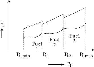
Fig.1. Incremental cost function with multiple fuels

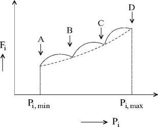
Fig.2. Fuel cost function with valve-point effect.

• 2.3.    ED problem with multiple fuels including valvepoint effect

The thermal unit cost function is non-convex, because of multi-valve steam turbines in generating units. Due to the valve-point effect, added sinusoidal terms to the second order cost functions as follows Eqn. (4). The generation function with multiple fuels (3) should be combined with valve-point effect (4), and objective function practically expressed as Eqn. (5), which is graphically shown in Fig.3.

^ak1^PGk + b kl P Gk + ^ck1 P Gk" "  P Gk "  ^PGki

^F = F C ( ^PGk ) = 1

^ak2^PGk + b k2^PGk + ^ck2

^PGk1 - ^PGk - ^PGk2

($ / h)

_ ^akn^PGk + b kn P Gk + c kn ^PGk(n - 1) ^- P Gk ^- P Gk

NG

F2 = FC (PG ) =2 (akPGk + bkPGk + ck ) + k=1

|e ck ^x sin( ^fck ^x (P Gmkn — P Gk ))|($/h)                   (4)

^ak1 ^P< 2k ⁺ b kl P Gk ^{+ c}k1 ⁺

|eckl x sin(fck1 x (Pmkn — PGk ))| ak2P<2k + bk2PGk + ck2 + min pGk - pGk - pGk1

F = 1

|eck2 ^{x sin(f}ck2 ^x (P mk"

—

P Gk ))| ^PGk1 ^- P Gk ^- P Gk2

.

aknPGk + bknPGk + ckn + max pGk(n—1) - PGk - PGk

| e ckn ^x s ^in(fckn ^x (PG™ ^— P Gk »|

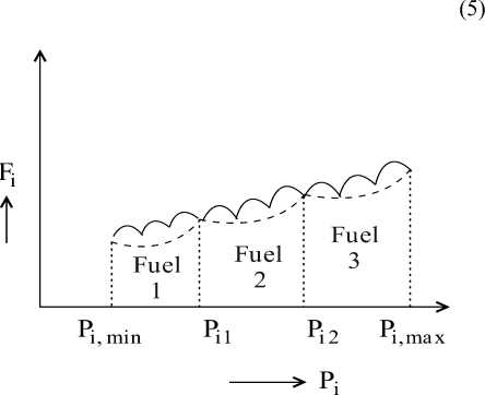
Fig.3. Fuel cost function with multiple fuels including valve-point effect.

• 2.3.1.    Equality constraint

Total generation of any power system must meet the required load demand and losses occur in the transmission lines as shown in Eqn. (6).

N _G

Z ^pGk = Pd + Pl            (6)

k = 1

Where PL denotes power losses and PD denotes the power demand. The power loss can be computed using B-coefficient method expressed as a second order function as shown in Eqn. (7).

nnn

Pl = ZZ P Gj B jk P Gk + Z B oj P Gj + B oo   (MW) (7)

j=1k=1j

• 2.3.2.    Power limit constraint

Any generator output can be varied between minimum and maximum power limits and follows Eqn. (8).

minmax

^PGk ^{- P}Gk ^{- P}Gk

• III.    Grey Wolf Optimization

• 3.1.    Searching for prey

• 3.2.    Encircling prey

Mirjalli presented the Grey Wolf Optimization (GWO) method [22] that is form on the trapping behaviour of the grey wolves (search agents) in nature. The ranking order follows as alpha (a) beta (в), omega (to), and delta (5) types of search agents. The grey wolves have different groups for different activities like making a group for staying, hunting the prey etc.

The hunting action initially started with some random initialization of search agents solutions from the search space. After the initialization search agents segregated based on their fitness values and recombine after they finding the prey.

After seeking a prey, search agents surround that prey and the surrounding behaviour can be mathematically represented by Eqn. (9) and Eqn. (10).

E = |O.X p (k) — X(k)|              (9)

X(k + 1) = X_p(k) — B.E           (10)

Here, k: the current iteration, B and O : are the coefficient vectors. Here B : used for sustain the distance between search agents grey wolves and prey. O represents disincentive in the hunting trail of the prey. Here, search agents position vector is represented by X and position vector of the prey is indicated byXp . The vectors B and O are computed as given in Eqn. (11) and Eqn. (12):

B = 2 x l x r j — 1                 (11)

O = 2 x r₂                   (12)

• 3.3.    Hunting

After surrounding the prey, search agents focus on hunting. The hunting is generally guided by a , в and to types of search agents. Among these, a provides the best candidate solution. Mathematically, hunting behaviour of search agents is formulated by (13)-

Ea=|(O1*Xa (k) ) — X(k)|(13)

Ep=|(O2*Xp (k) ) — X(k)|(14)

• E„=|( Оз*Хю (k)) — X(k)|(15)

• 3.4.    Attacking prey

X1 = Xa (k) — ( B1*Ea)

X2 = Xp (k)-(B2*Ep)

X3 = Xto (k)-(Вз*Ёю)

X(k +1) = (X1 + XX2 + X3)(19)

After completion of hunting, search agents attack the prey. Based on the position of a , p and to grade search agents, the GWO method allows the search agents, i.e. search agents to update their positions to attack the prey. In order to approach the prey, two parameters aandAare considered. Here, a decreases linearly from 2 to 0 as the iterations increase and variations of A are also decline witha .

• IV.    Numerical Results

  The potency of the suggested algorithm for practicable appliance has been applied on ten units system. The test system having four cases and description of case studies for simulation are presented in Table 1. The input data from K.Vaisakh [20]. In this ED problem, generators are supplied with three types of fuels, namely 1, 2 and 3. The total ten units are categorized into three subsystems, where the 1^st subsystem consists of four thermal units and remaining two subsystems consists of three thermal units. Among the ten thermal units, unit-1 is supplied with only two types of fuels (1 and 2), unit-9 is a different, even though fuel 2 is available but uneconomical to burn and when fuels 1 and 3 are not available then fuel 2 can be utilized instantly. The population and maximum iteration (termination criteria) are set as 40 and 500. To reduce the statistical errors, test system is repeated 20 times and all simulations are developed in MATLAB 2014a.

• 3.5.    Implementation of GWO for the ED problem

The implementation steps to ED problem by using GWO algorithm are shown below.

Implementation steps of the GWO algorithm in ED problem:

Step 1   Initialization

• (a)   Read cost coefficients, valve-point loading

Coefficients and B coefficients.

• (b)    Set power limits of each generator output.

• (c)    Set number of search agents and maxiter.

• (d)    Read GWO parameters: upper, lower limits of Search space.

Step 2 Initially the locations of the a , p and to , Initial fitness values randomly chosen as follows.

Alpha_pos=zeros(1,dim); Alpha_score=inf;

Beta_pos=zeros(1,dim); Beta_score=inf;

Omega_pos=zeros(1,dim); Omega_score=inf;

Positions=rand(SearchAgents_no,dim).*(ub-lb)+lb;

Step 3 Set the step time t=0

Step 4 Calculate the initial positions of the fitness Function. Set the previous finest position of each Alpha to his presant position.

Step 5 Let t=t+1

Step 6 Select the associate of each alpha and calculate the fitness function for each alpha

Step 7 Revise the chronological best position among the search agents and previous finest position of each alpha.

Step 8 Repeat from Step 6, to obtain best value For objective function upto max. Iteration.

Table 1. Different case studies for Test power system

Test power system	case	Demand power (MW)	Valvepoint loading	Transmission losses	Multiple fuels
	1	2400 to 2700 2400 to	X	X	✓
	2
10-unit		2700 2400 to	✓	X	✓
	3
		2700 2400 to	X	✓	✓
	4	2700	✓	✓	✓

4.1. Case 1

Table 2. power outputs and fuel types for case I of test system by GWO

Unit	2400 MW		2500 MW		2600 MW		2700 MW
	F	P(MW)	F	P(MW)	F	P(MW)	F	P(MW)
1	1	189.7659	2	206.4777	2	209.8288	2	218.2171
2	1	202.3233	1	206.4904	1	207.9304	1	211.7013
3	1	254.0453	1	265.8287	1	269.9086	1	280.7045
4	3	233.0460	3	235.9228	3	236.9606	3	239.6168
5	1	241.9131	1	258.0950	1	263.8418	1	278.4173
6	3	233.0691	3	235.9700	3	237.0033	3	239.6154
7	1	253.2479	1	268.9370	1	274.3034	1	288.6629
8	3	232.9886	3	235.9567	3	236.9979	3	239.6414
9	1	320.3758	1	331.5210	1	402.8262	3	428.4983
10 PT	1	239.2249 2400	1	254.8006 2500	1	260.3989 2600	1	274.9251 2700
Cost($/h)		481.7226		526.2388		573.7413		622.8092

Here, the cost functions of 10 units system is only with multiple fuels. This case, the 10-unit system data, such as fuel types and its cost coefficients are taken from C.E.Lin [8]. Initially, the load demand is considered as 2400 MW and later with increment of 100 MW, load demand increases up to 2700 MW. The GWO method is essential to meet one power balance equality constraint and 20 powers limits inequality constraints of the system. The optimal generation schedule and selection of fuels among 20 individuals run for case I by the GWO for various demands of 2400 MW to 2700 MW are presented in Table 2.

Table 3. Comparison of optimization methods for case I of test system

Demand (MW)	2400	2500	2600	2700
Methods	Minimum Cost ($)
HM [8]	488.500	526.700	574.030	625.180
MHNN [9]	487.87	526.13	574.26	626.12
AHNN [10]	481.700	526.2300	574.370	626.240
MPSO [11]	481.723	526.239	574.381	623.809
PSO [19]	481.723	526.240	574.381	623.8094
DE [19]	481.723	526.239	574.381	623.8098
IPSO [19]	481.7226	526.2388	574.380	623.8089
SDE [20]	481.7226	526.2388	574.3808	623.8092
SFLA-GHS [20]	481.7226	526.2388	574.3808	623.8092
GWO	481.7226	526.2388	573.7413	622.8092

The finest outcomes of GWO in 20 trails is correlated with hierarchical economic dispatch [8], HNN [9-10], PSO [11, 19], DE [19], IPSO [19], SDE [20] and SFLA-GHS [20] given in Table 3. The results presented in the Table 3 proved that the suggested GWO provides the better solution aspect than others methods. For 2400 MW and 2500 MW IPSO [19], SDE [20] and SFLA-GHS [20] methods produce the same optimal cost as proposed GWO method, as the power demand increases GWO produce slightly better results as compared to other methods. From the results presented in Tables 2 and 3conclude that the suggested GWO is more competent compared to other methods reported in literature.

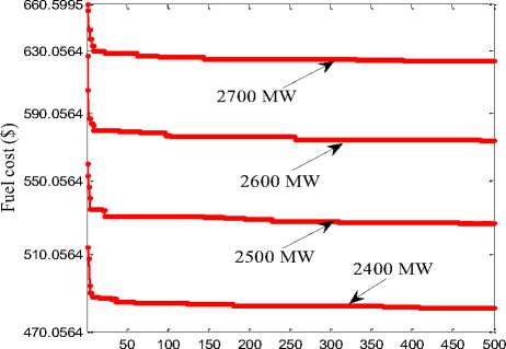
Fig. 4 has shown the convergence aspects for case I of test system for various power demands 2400 MW to 2700 MW. The simulation outcomes found that the costs, fuel types and dispatch levels from GWO are quite similar to that of IPSO [19], SDE [20] and SFLA-GHS [20] methods and diverse from other methods. The global achievement of GWO is always superior to practical ED problems than other existing methods.

• 4.2.    Case II

  The ED problem with multiple fuels including valvepoint effect is treated as case II. The 10-units system data such as fuel types and its cost coefficients are taken from Mostafa Kheshti [17]. Power demands are examine as similar to earlier case like 2400 MW to 2700 MW with addition of 100 MW. The optimal generation of schedule and selection of fuels among 20 individual runs for case II by the GWO for demand load demands of 2400 MW to

  2700 MW with stepwise increment of 100 MW is presented in Table 4.

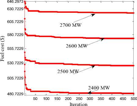
Fig.4. GWO Convergence characteristics for case I with various load demands

Table 4. power outputs and fuel types for case II of test system

Unit	2400 MW		2500 MW		2600 MW		2700 MW
	F	P(MW)	F	P(MW)	F	P(MW)	F	P(MW)
1	1	188.3723	2	205.5101	2	208.5495	2	217.6101
2	1	204.7311	1	207.7723	1	209.2377	1	213.1885
3	1	254.2863	1	262.8788	1	268.4265	1	282.9418
4	3	234.2656	3	237.0844	3	237.2194	3	238.2967
5	1	241.6210	1	258.7284	1	264.9852	1	282.6130
6	3	231.0348	3	234.1271	3	237.7589	3	240.5764
7	1	253.5449	1	266.2820	1	273.2244	1	284.1752
8	3	231.9787	3	237.4925	3	236.5563	3	241.3828
9	1	321.5086	1	333.1468	1	402.4569	3	424.0150
10	1	238.6567	1	256.9777	1	261.5852	1	275.2006
PT		2400		2500		2600		2700
Cost($/h)		481.9501		526.4319		573.8869		622.9597

For case II, the optimal solution attained from the methods informed in the literature namely, DE [19], PSO [19], IPSO [19], SDE [20], MSFLA [20], GHS [20], SFLA-GHS [20] and the suggested algorithms are listed in Table 5. The proposed GWO obtain optimal cost for various power demands than other approaches. Due to the additional sinusoidal term in the cost function, for all demands the fuel costs are increased.

From Table 5 it is evident that the suggested GWO provides the finest solution quality than others approaches. For 2400 MW and 2500 MW GHS [20] and SFLA-GHS [20] methods are produce slightly better optimal cost as compare with proposed GWO method, as the power demand increases the GWO produces better results as compare with other methods. The outcomes in Tables 4 and 5, conclude that the GWO is more competent to other methods narrated in literature. Fig. 5 showed the convergence aspects of case II for various load demands 2400 MW to 2700 MW.

Table 5. Comparison of optimization methods for case II of test system

Demand	2400 MW	2500 MW	2600 MW	2700 MW
Methods	Minimum Cost ($)
DE [19]	482.1245	527.0024	574.9744	624.4606
PSO [19]	482.0014	526.9336	574.7146	624.2449
IPSO [19]	481.8044	526.2929	574.4326	623.8730
SDE [20]	481.7305	526.24266	574.3839	623.8375
SFLA [20]	482.278	526.33166	574.89446	623.9016
GHS [20]	481.75043	526.26547	574.78857	623.6217
SFLA-GHS [20]	481.7754	526.32577	574.4561	623.8406
GWO	481.9501	526.4319	573.8869	622.9597

Iteration

Fig.5. GWO Convergence characteristics for case II with various load demands

• 4.3.    Case III

  To demonstrate the potency of the suggested algorithm enveloping the transmission losses to the Case I, it can be considered as Case III. This case, the 10-units system data such as fuel types and its cost coefficients are taken from C.E.Lin [8], loss coefficients taken from J.S. Dhillon [21]. Case III also implemented on different power demands from 2400 MW to 2700 MW with addition of 100 MW. Due to the addition of transmission losses to the power demand the fuel cost increases. For case III, the optimal power outputs and selection of fuels for various power demands attained from the GWO method are presented in Table 6.

• 4.4.    Case IV

  The ED problem with multiple fuels including valvepoint effect along with transmission losses is considered as case IV. In this case, the 10-units system data, such as fuel types and the cost coefficients are taken from Mostafa Kheshti [17] and loss coefficients taken from J.S.Dhillon [21]. Load demands are consider as similar to previous case like 2400 MW to 2700 MW with addition of 100 MW. The Case IV study on test system briefly explains about the practical considerations in the power system because it consist multiple fuels, valve point loading and losses. The fuel cost increased for all demands due to the effect of additional constraints. The proposed GWO obtained economic cost for various power demands than other approaches and optimal combination of generator outputs, fuel type for test system presented in table 7. For the case IV proposed method obtained optimal cost 698.5726 ($/h), but

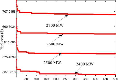
  Synergic predator-prey optimization [21] provides optimal cost 700.776 ($/h) for 2700 MW power demand. Fig. 7 showed the convergence characteristics of case IV for different load demands of 2400 MW to 2700 MW.

Most of the researchers should not perform the multiple fuels ED along with transmission losses for various power demands like 2400 MW, 2500 MW and 2600 MW. This is one of the main contributions in the presant work. The proposed GWO obtain optimal cost for 2700 MW power demand than other methods. For the case III proposed method obtain optimal cost 698.3317 ($/h), but Synergic predator-prey optimization [21] provides optimal cost 700.296 ($/h) for 2700 MW power demand. Fig. 6 showed the convergence aspects of case III for different load demands of 2400 MW to 2700 MW.

Table 6. Optimal generations and fuel types for case III of test power system by GWO

Unit	2400 MW	2500 MW	2600 MW	2700 MW
F	P(MW)   F	P(MW)	P(MW)	F  P(MW)
1     2	206.2335   2	210.4448	219.7385	2   231.1912
2     1	207.3595    1	209.2966	213.5517	1   218.7948
3      1	267.9580   1	273.5761	285.7673	1   300.8213
4    3	236.7507   3	238.1490	241.2047	3   244.9550
5      1	261.4620   1	269.2574	285.9026	1   306.3561
6     3	236.8098   3	238.2211	241.2750	3   245.0627
7     1	271.0914   1	278.3888	294.3393	1   313.9002
8     3	236.4211   3	237.7907	240.8021	3   244.5081
9     1	331.1212   3	403.5331	431.2478	3   440.0000
10     1	254.0294   1	261.3991	276.9927	1   296.1998
P loss	109.2365	120.0566	130.8218	141.7890
PT	2509.236	2620.056	2630.821	2841.789
Cost($/h)       530.5528		583.3682	638.6178	698.3317

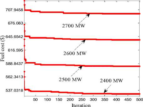
Fig.6. GWO Convergence characteristics for case III with various load demands.

Table 7. Optimal generations and fuel types for case IV of test power system by GWO

Unit	2400 MW		2500 MW		2600 MW		2700 MW
	F	P(MW)	F	P(MW)	F	P(MW)	F	P(MW)
1	2	207.389	2	212.305	2	220.737	2	230.7157
2	1	208.734	1	209.200	1	211.692	1	218.3920
3	1	264.496	1	270.454	1	287.713	1	302.2410
4	3	235.613	3	237.622	3	241.245	3	245.8280
5	1	257.485	1	268.356	1	287.187	1	304.8487
6	3	237.891	3	238.695	3	242.061	3	244.6187
7	1	274.261	1	280.107	1	291.375	1	309.3022
8	3	236.141	3	237.493	3	241.119	3	246.0893
9	1	332.616	3	405.971	3	431.034	3	440.0000
10	1	254.674	1	259.909	1	276.643	1	299.8028
P loss		109.304		120.118		130.811		141.8383
PT		2509.30		2620.11		2630.81		2841.838
Cost($/h)		530.7738		583.5511		638.8057		698.5726

Iteration

Fig.7. GWO Convergence characteristics for case IV with various load demands.

• V. Conclusions

In this paper, Grey Wolf Optimization method has been proposed and implemented for finding the economic dispatch with various fuels and valve-point loading. While searching for a better solution, GWO does not obligate any statistics about the gradient of the fitness function. The GWO method was proved on 10-units system with four different case studies and four different power demands. The major contribution of the present work was including transmission losses to the test system for various power demands. The outcomes were correlated with other approaches described in the literature and indicated that GWO had faster convergence aspects, improved cost results, dominant computing efficiency and more cognizant accomplishment. The GWO method can be a viable approach to reduce the cost and increases the efficiency for a power grid by providing best power outputs and economic fuel selections. The GWO method is a promising solution for solving complicated non-smooth optimization problems in large scale power system.