Hafnian of some three-parameter Toeplitz matrices and perfect matchings of arc and chord diagrams

Let A = ( a ij ) be a symmetric matrix of even order n over a commutative associative ring. The hafnian of A is defined as

HAFNIAN OF SOME THREE-PARAMETER TOEPLITZ MATRICES AND PERFECT

MATCHINGS OF ARC AND CHORD DIAGRAMS

Institute of Physics and Mathematics, Federal Research Centre Komi Science Centre, Ural Branch, RAS, Syktyvkar

^{Hf( A} )=       52       a i 1 i 2 '•• a i n - 1 i n ,

( i 1 i 2 |...|i n - 1 i n )

where the sum runs over all partitions of the set { 1 , 2 ,..., n} into disjoint pairs ( i 1 i 2 ) , ... , ( i n- 1 i n ) up to the order of pairs, and the order of elements in each pair. So, if n = 4 then Hf ( A ) = a 12 a 34 + a ₁₃ a 24 + a 14 a 23 . The hafnian of the empty matrix is taken to be 1 .

Recall that a matrix is called Toeplitz if all its diagonals parallel to the main diagonal consist of the same elements. A symmetric Toeplitz matrix is uniquely determined by its first row. Let a, b, c be real or complex numbers. We denote by T m ( a, b, c ) the symmetric Toeplitz matrix of order 2 m with zero main diagonal whose first row has the form (0 , a,b, b,..., b, c ) or (0 , a ) if m = 1 . For example (dots denote zeros),

T з ( a, b, c ) =

a b b b c

a  b  b  bc

•   a   b   bb a • abb ba  •  ab b   b   a   •b b   b   b   a•

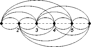
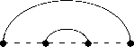
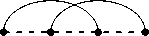
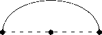
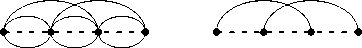
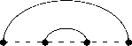
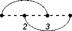
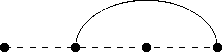
In the first part of our work, we obtain an explicit formula for exact calculating the hafnian of such matrices. Using this formula, we also give an asymptotic estimate. In the second part, we consider sequences of values Hf(Tm (a, b, c)) with respect to m for non-negative integers a, b, c. Such sequences can be interpreted in the language of graph theory as follows. It is easy to see that if M is the adjacency matrix of an unordered multigraph with even number of vertices, then Hf(M) equals the total number of perfect matchings of the multigraph. We denote by Gm(a, b, c) the multigraph with 2m vertices whose adjacency matrix is Tm (a, b, c). It is convenient to represent such a multigraph in the form of an arc or chord diagram. An arc diagram is a graph presentation method where all the vertices are located along a line in the plane, while all edges are drawn as arcs. The vertices of a chord diagram are located on a circle and edges are chords of the circle. However, if a pair of vertices of a chord diagram is joined by several edges, then to distinguish them in a figure, we will draw them not in the form of segments, but also in the form of arcs. By construction, the vertices 1 and 2m of the diagram Gm(a, b, c) are joined by c edges, vertices with numbers differing by one are joined by a edges, and all other pairs of vertices are joined by b edges (see Figure 1).

order n . Then

n/ 2

Hf( A + B ) = X X Hf( A [ a ])Hf( B {a} ) . (1) k =0 ^a ^Q 2 k,n

Consider the matrix T _m ( a, b, c ) , m >  2 . For brevity, we denote it now by A m :

	(	0 a	a . . .	b ··· .. ..	b	c
						b
m =		b	. . .	.. ..	. . .	. .	, m >  2 .
		. .	. . .	.. ..	. . .	b
		b		.. ..	. . .	a
		c	b	··· b	a	0
|				{Z			}

2 m

(a)

This matrix can be represented as the sum of the following two matrices:

B m

a

b

.

.

.

\

.

.

.

b

43 (b)

Fig. 1. Arc (a) and chord (b) diagrams G 3 (2 , 1 , 0).

Рис. 1. Дуговая (a) и хордовая (b) диаграммы G з (2 , 1 , 0).

.

.

.

\

-b

a b ...... b\

..

....

...

.... .    .    ...

.                     .                     ..

,

..    ...    ...    ...

..           ....

..... b a 0 /

........ 0    c — b \

..

.. .. ..

.. ..

..

. ^. ..

..

0 ......... 0   /

It has shown in [4], that if we put 0 ⁰ = 1 then the hafnian of B m can be calculated by the following formula:

Thus, in the second part of our work, we consider sequences of numbers of perfect matchings of the multigraphs G m ( a, b, c ) for some values of a, b, c .

Note that in many papers (see, for example, [1,2]), chord diagrams are understood to be perfect matchings of chord diagrams in our terminology, and perfect matchings of arc diagrams are called linear chord diagrams . In the same papers, one can find references to extensive applications of these structures.

1. The hafnian of three-parameter Toeplitz matrices

Let Q k _,n denote the set of all unordered k -ele-ment subsets of the set { 1 , 2 ,..., n} . Let A be a matrix of order n and α ∈ Q k,n . We denote the submatrix of A formed by the rows and columns of A with numbers in a by A [ a ] , and the submatrix of A formed from A by removing the rows and columns with numbers in α by A{α} . The following property proved in [3]:

Proposition 1. Let A , B be symmetric matrices of even

^Hf( B m ) = g( a - b ) m-k ^b k k (2)

In other words, the value of the hafnian of such a matrix is equal to the value of the polynomial

P m ( Х,У )

m

^X k =0

( m + k )! k !( m — k )

-k

in two variables x,y at x = b and y = a — b . Note that for y = 1 this polynomial coincides with the Bessel polynomial of degree m [5]. Using (1), we find

m

Hf ( A m ) = ]T   ]T    Hf ( B m [ a ]) Hf ( C m {a} ) .

k =^{0 a} EQ 2 k, 2 m

If a = (1, 2, . . . , 2m), then Cm {a} is the empty matrix and Hf( Cm {a}) = 1. If a = (2,3,..., 2 m — 1), then Hf(Cm{a}) = Hf(Cm[1,2m]) = c — b. In all other cases, Hf(Cm{a}) = 0. It follows that

By induction on k , it can be proved that

Hf ( A _m ) = Hf ( B _m ) + ( c —

m

b ) Hf ( B m- 1 ) =

= ^2( a - b ) ^{m - k} b ^k

k =0 m- 1 ^{+ (} c — ^b ) X ⁽ a — ^b ) l =0

( m + к )! к !( m — к )!2 ^k

0 <  U к !

2 ^k m !(2 m — к )! \ (2 m )!( m — к )! /

≤

m-l- 1 b l ⁽ m ^{+ l — 1)!}

l !( m — l — 1)!2 ^l'

Hence,

Performing simple transformations, we finally obtain

Hf ( A m ) =

(2 m )! / b

“ 2( к — 2)!(2 m — 1) ’

2 < к < m.

m- 1

+ X (a k=0

-

m !    2

_{b )} m - k - 1 "fc!

m

+

b\k ((    (mm + ^ )!

2) v a^—bfm—f. ⁺

.    ,. ( m + к — 1)!\

+( c — b )(---- ^4) • (4)

( m — к — 1)! /

If a = b, then the first summand can also be entered under the sum sign:

Hf ( A m )

_ X ( a — b ) ^{m - k - 1}

=            k!

k =0

S    bm(2m)! X (a — b)k m    m !2m       bk к!   < k=0

|b| ^m (2 m )! X |a — b| ^k /    2 ^k m !(2 m — к )!\

< m !2 ^m   k=₂ \b\ ^k к ! \ — (2 m )!( m — к )! ) <

|b| ^m (2 m )!     X |a — b| ^k

< m !2 ^{m +1} (2 m — 1) k=2 |b| ^k ( к — 2)! <

< ^|b| m^{- 2 (2 m )! |a — b| 2} e |a-b|/|b|

- m !2 ^{m +1} (2 m — 1)          ’

Similarly,

( m + к — 1) ( m — к )!

( m ( a + c — 2 b ) + к ( a — c )) J .

S m-

m- 1

= E( a — k=0

b . k b ^{m - k -} 1 (2m — к — 2)! ) к !( m — к — 1)!2 ^{m - k - 1}

Remark 1 . Using (4) and (5), one can compute Hf( A m ) in time O ( m ) .

The obtained formulas allow us to give an asymptotic estimate for Hf ( A m ) .

Proposition 2. If b = 0 , then Hf( A m ) = a m^- 1 ( a + c ) .

If b = 0 , then

Hf( A m ) - ( m ( b ) e ^{( a - b} ) ^/b , m ^^ m !    2

b ^m (2 m )!

m !2 ^m

m- 1

X k=0

( a — b ) ^k 2 ^{k +1} m !(2 m — к — 2) b k +¹ к !(2 m )!( m — к — 1)!

bm(2m)! XV    (a — b)k     Л 2m — 2i m!2m      I bk+1 к!(2m — к — 1) ^ 2m — i k=0 \ v             ' i=1

Proof. If b = 0 , then nonzero summands in (3) correspond only to the values к = 0 and l = 0 . Therefore, in this case Hf( A m ) = a m^- 1 ( a + c ) .

In the case b = 0 , the proof is similar, with slight modifications, to the proof of the asymptotic formula for Bessel polynomials in [6]. We introduce for convenience the notation

It follows that

|S . < |b|m- 1(2m)! m-1 |a — b|k < m 1 —   m !2 mm   k—0 |b|kk! -

< IblTZEm)! ea-b/b| m !2 mm

Now we can write the following chain of inequalities:

,    ,    ⁽² m ^)!

f m ^{( Х,}У ) = ---Г- m !

m

e y/x _.

| Hf ( A _m ) — f _m ( b, a — b ) | =

Our task is to show that Hf( A m ) — f _m ( b, a — b ) as m → ∞ . In the course of the proof, for the sake of convenience, we also denote Hf( B _m ) by S _m . If we replace k by m - k under the summation sign in (2), and then take out the first summand as a common factor, we get:

S _m + ( c — b ) S _{m -} 1 —

b ^m (2 m )! X ( a — b ) ^k m !2 ^m         b k к !

k =0

≤

m

Sm = E( a — b) k bm-k k=0

(2 m — к )!

b ^m (2 m )! m !2 ^m

m

X k=0

к !( m — к )!2 ^{m - k}

( a — b ) ^k 2 ^k m !(2 m — к )! b k к !(2 m )!( m — к )!

b ^m (2 m )! — ( a — b ) ^k

< Sm    m!2m       bkк!   + k=0

+ 1           M |b| ^m (2 m )! X |a — bV^£_<

+ |c — b||Sm-11 + m!2m    E -bbfckT < k=m+1 1 1

< f m ( H |a — b| )

/     |a — b| ²

\ 2(2 m — 1) |b| ²

+

|c-b| m|b|

Hence,

By Proposition 2

Hf(Am)     . _ |Hf(An ) — fm (b,a - b) | < fm(b,a - b) " = Ifm(b,a - b)|      <

• < f m ⁽ Ibl, ^{|a - b|} ) /     ^{|a - b|} 2      + ^{|c - b|} , Л

• - f m ( b,a - b ) | \2(2 m - 1) |b| ²     m|b|      .'

a m ^∼

(2 m )!

e m!2m

The ratio f _m ( |b|, |a - b| ) /f _m ( b, a - b ) | is a constant, and the expression in brackets approaches zero as m increases. This completes the proof.

Remark 2 . The inequality (6) guarantees fast convergence only for small values of the ratios |c - b|/|b| and |a - b|/|b| .

Remark 3 . The value of the parameter c affects only the convergence rate, but does not affect the form of the asymptotic behavior of Hf ( A m ) . This is not surprising, since the parameter c , in contrast to the parameters a and b , corresponds to only two elements of a matrix.

For non-negative integers a, b, c , formulas obtained in this section allow us to calculate exactly and approximately the values of the number of perfect matchings of arc and chord diagrams G _m ( a, b, c ) . Further we will consider some concrete examples.

2. Perfect matchings of some diagrams G _m ( a, b, c )

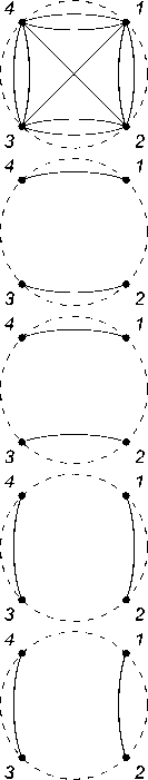
2.1. The arc diagram G m (2 , 1 , 1)

Let us consider the arc diagram Gm(2, 1, 1). Neighboring vertices are joined in it by two arcs (we call them conditionally «upper» and «lower» arc), and any other pair of vertices is joined by one arc (see Fig. 2). Let am denote the number of perfect matchings of Gm(2, 1, 1). From (5) we get am = Hf(Tm2,1,i)) = X k22k (m - k);. (7) k=0

Applying (7) for consecutive m , we get the sequence A 001515 from [7]. Thus, we have a new interpretation of this sequence.

If we remove «lower» arcs in the diagram G m (2 , 1 , 1) , then we get the complete graph K 2 m . The number of perfect matchings of K 2 _m equals (2 m )! /m !2 ^m . So, it follows from (8) that adding «lower» arcs joining neighboring vertices to the arc diagram of the complete graph increases the number of perfect matchings by approximately e times.

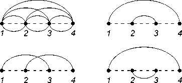
It is known from the description of the sequence A 001515 in [7] that its m -th term is equal to the number of partitions of the sets { 1 , 2 ,..., k} , m < k <  2 m , into m non-empty blocks with no more than two elements per block. For example, if m = 2 , then we get partitions: { 1 , 2 } , { 13 , 2 } , { 13 , 24 } , { 1 , 23 } , { 14 , 23 } , { 12 , 3 } , { 12 , 34 } — 7 in total. We establish now the correspondence between the given interpretation of this sequence and its interpretation through the number of perfect matchings of the arc diagram G _m (2 , 1 , 1) obtained above. As an example, Figure 2 illustrates the arc diagram G 2 (2 , 1 , 1) and all its perfect matchings.

We assign a partition to each perfect matching by the following rule. If two vertices are joined by an «upper» arc, then we put down their numbers to the same block. If two neighboring vertices are joined by an «lower» arc, then we «glue» them into one, renumber vertices of the obtained graph from left to right and put down the number of a single vertex to a separate block (see Fig. 3). Carrying out this procedure in the opposite direction, we will uniquely restore the perfect matching of the diagram for a given partition. The given scheme obviously works for an arbitrary m .

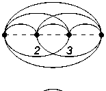
2.2. The chord diagram G m (2 , 1 , 2)

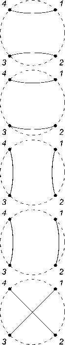
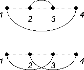
Consider the chord diagram G _m (2 , 1 , 2) . Neighboring vertices are joined in it by two chords, and any other pair of vertices is joined by one chord (see Fig. 4).

Let b m denote the number of perfect matchings of G _m (2 , 1 , 2) . It follows from the above that

b m = ^Hf ( T m (21 , ² )) = m X                  .

k =0

By Proposition 2

b _m

∼

(2 m )!

m !2 ^{m e}'

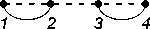
Fig. 2. The arc diagram G 2 (2 , 1 , 1) and its perfect matchings.

Рис. 2. Дуговая диаграмма G 2 (2 , 1 , 1) и ее совершенные паросочетания.

Setting b 1 = 2 and using (9) for consecutive m >  2 , we get the sequence A 336400 from [7]. This sequence is also presented in the second column of Table 1. It is easy to see, that sequences ( a _m ) and ( b _m ) are connected to each other by the following relation:

^b m = a m + a m- 1 . ⁽¹⁰⁾

Indeed, the diagram Gm (2, 1,2) differs from Gm(2, 1, 1) by only one edge joining the vertices 1 and 2m. For Gm(2, 1, 2), the number of perfect matchings, in which vertices 1 and 2m are joined by an edge, equals am-1. Hence, bm is greater than am by am-1.

{ 14 , 23 }

{ 13 , 24 }

{ 12 , 34 }

{ 1 , 2 }

{ 13 , 2 }

{ 12 , 3 }

{ 1 , 23 }

Fig. 3. The correspondence of two interpretations of the sequence A 001515.

Рис. 3. Соответствие двух интерпретаций последовательности A 001515.

From the equalities (10) and (11), we can derive the following recurrence relation for terms b _m :

b m +i = 2 mb m + (2 m - 2) b _m — 1 + b _m — 2 , m >  4 .

and

(4m2 - 3)bm + (2m + 1)bm-1     . „ bm+1 = -----------о-----:-----------, m > 3.

2 m - 1

2.3. The arc diagram G m (2 , 1 , 0)

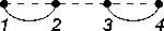
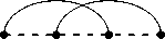
Let us consider the arc diagram G m (2 , 1 , 0) . Neighboring vertices are joined in it by two arcs, the vertices 1 and 2 m are not adjacent if m >  2 , and all other pairs of vertices are joined by one arc (see Fig. 5).

1234 1234

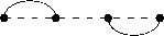
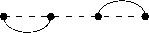
Fig. 5. The arc diagram G 2 (2 , 1 , 0) and its perfect matchings.

Рис. 5. Дуговая диграмма G 2 (2 , 1 , 0) и ее совершенные паросочетания.

Let c _m denote the number of perfect matchings of G _m (2 , 1 , 0) . From (5) we get

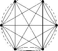
Fig. 4. The chord diagram G 2 (2 , 1 , 2) and its perfect matchings.

Рис. 4. Хордовая диаграмма G 2 (2 , 1 , 2) и ее совершенные паросочетания.

C m = Hf( T 2m (2 , 1 , 0)) =

m

= X k=1

1     ( m + k — 1)

( k - 1)!2 ^{k - 1}    ( m - k )!

It is known that the sequence ( a m ) satisfies the following recurrence relation:

By Proposition 2

a m = (2 m - 1) a m- 1 + a m— 2 , a 1 = 2 , a 0 = 1 . (11)

c m ^∼

(2 m )!

e m!2m

Setting c 1 = 2 and using (12) for consecutive m >  2 , we get the sequence presented in the third column of Table 1.

As in the case of ( a m ) , the sequence ( c m ) can be interpreted through partitions of finite sets of natural numbers into blocks. Namely, c _m is equal to the number of partitions of sets { 1 , 2 ,... ,k} , m < k <  2 m , into m non-empty blocks so that there are no more than two elements in each block and there is no block containing 1 and k simultaneously. For example, if m = 2 then we get partitions: { 1 , 2 } , { 13 , 24 } , { 1 , 23 } , { 12 , 3 } , { 12 , 34 } — 5 in total.

It is easy to see that sequences ( a m ) and ( c m ) are connected to each other by the following relation:

1  23  4

c m    a m   a m- 1 •

1  23  4

1  23  4

Indeed, the diagram G m (2 , 1 , 1) differs from G m (2 , 1 , 0) by only one edge joining the vertices 1 and 2 m . For G m (2 , 1 , 1) , the number of perfect matchings, in which vertices 1 and 2 m are joined by an edge, equals a _{m - 1} . Hence, a _m is greater than c _m by a _{m - 1} . From the equalities (11) and (13), one can derive the following recurrence relation for terms c _m :

C m +1 = (2 m + 2) C m - (2 m - 4) C m- 1 - C m- 2 , m >  4 .

and

C m +1 ⁼

(4 m ² + 1) C m + (2 m + 1) C m— 1

2 m — 1

m >  3 .

Starting from m = 2 , C m coincides with the ( m — 1) -th term of the sequence A 144498 from [7]. Thus, one can say that we get a new interpretation of A 144498 .

• 2.4.    The arc diagram G m (1 , 2 , 2)

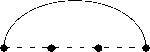
Let us consider the arc diagram G m (1 , 2 , 2) . Neighboring vertices are joined in it by one arc, and any other pair of vertices is joined by two arcs (see Fig. 6). Let u _m denote the number of perfect matchings of G _m (1 , 2 , 2) . From (5) we derive that

U m = Hf( T 2 m (1 , 2 , 2)) = X < — !p m + k ) . k ! ( m — k )!

⁼ (14)

Setting u 1 = 1 and using (14) for consecutive m , we get the sequence presented in the first column of Table 2. Elements of this sequence coincide in absolute value with the corresponding elements of the sequence A 002119 from [7].

Fig. 6. The arc diagram G 2 (1 , 2 , 2) and its perfect matchings.

Рис. 6. Дуговая диаграмма G2(1,2,2) и ее совершен- ные паросочетания.

By Proposition 2

u m ~

(2 m )! em m !

If one joins in the diagram G _m (1 , 2 , 2) neighboring vertices by additional «lower» arcs, then we obtain the diagram G _m (2 , 2 , 2) . It is nothing more than a complete multigraph, each pair of vertices of which is joined by two edges. It is not difficult to calculate that the number of perfect matchings of such a graph equals (2 m )! /m ! . From (15) it follows that, by appending additional «lower» arcs joining neighboring vertices to the diagram G _m (1 , 2 , 2) , we get the number of perfect matchings increased by approximately ^e times.

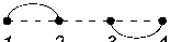
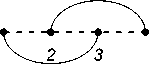
Now we derive a recurrence for the sequence ( u _m ) . For G _m (1 , 2 , 2) , consider perfect matchings, in which the vertex 2 m is joined by an arc with the vertex 2 m — 1 . It is obvious that the number of such perfect matchings equals u _{m - 1} . Consider a perfect matching, in which the vertex 2 m is joined by an «upper» arc with the vertex 2 m — 2 (see Fig. 7(a)). The remaining 2 m — 2 vertices can be paired in at least u _{m - 1} ways. But the vertices 2 m — 1 and 2 m — 3 are considered here as neighboring, and therefore they assume only one variant of the connection (by an «upper» arc), although if we consider the diagram G 2 _m (1 , 2 , 2) in general, this vertices can be joined by two different arcs. Thus, one must also take into account perfect matchings, in which the vertices 2 m — 1 and 2 m — 3 are joined by a «lower» arc (see Fig. 7(b)). The number of such matchings is obviously u _{m - 2} .

2m-3   2m-2   2m-1 2m

(a)

Fig. 7. A derivation of a recurrence for ( U m ).

Рис. 7. Вывод рекуррентного соотношения для ( U m ).

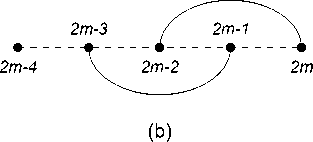
Table 1

The number of perfect matchings of multigraphs G m ( a, b, c )

Таблица 1

Число совершенных паросочетаний мультиграфа G m ( a,b, c )

m	G m (2 , 1 , 1)	G m (2 , 1 , 2)	G m (2 , 1 , 0)
1	2	2	2
2	7	9	5
3	37	44	30
4	266	303	229
5	2431	2697	2165
6	27007	29438	24576
7	353522	380529	326515
8	5329837	5683359	4976315
9	90960751	96290588	85630914
10	1733584106	1824544857	1642623355
11	36496226977	38229811083	34762642871
12	841146804577	877643031554	804650577600
13	21065166341402	21906313145979	20224019536825
14	569600638022431	590665804363833	548535471681029
15	16539483668991901	17109084307014332	15969883030969470
16	513293594376771362	529833078045763263	496754110707779461
17	16955228098102446847	17468521692479218209	16441934503725675485
18	593946277027962411007	610901505126064857854	576991048929859964160
19	21992967478132711654106	22586913755160674065113	21399021201104749243099
20	858319677924203716921141	880312645402336428575247	836326710446071005267035

Table 2

The number of perfect matchings of multigraphs G m ( a, b, c )

Число совершенных паросочетаний мультиграфа G m ( a, b, c )

Таблица 2

m	G m (1 , 2 , 2)	G m (1 , 2 , 1)	G m (1 , 2 , 0)
1	1	1	1
2	7	6	5
3	71	64	57
4	1001	930	859
5	18089	17088	16087
6	398959	380870	362781
7	10391023	9992064	9593105
8	312129649	301738626	291347603
9	10622799089	10310669440	9998539791
10	403978495031	393355695942	382732896853
11	16977719590391	16573741095360	16169762600329
12	781379079653017	764401360062626	747423640472235
13	39085931702241241	38304552622588224	37523173542935207
14	2111421691000680031	2072335759298438790	2033249827596197549
15	122501544009741683039	120390122318741003008	118278700627740322977
16	7597207150294985028449	7474705606285243345410	7352204062275501662371
17	501538173463478753560673	493940966313183768532224	486343759162888783503775
18	35115269349593807734275559	34613731176130328980714886	34112193002666850227154213
19	2599031470043405251089952039	2563916200693811443355676480	2528800931344217635621400921
20	202759569932735203392750534601	200160538462691798141660582562	197561506992648392890570630523

The same is true for perfect matchings, in which the vertex 2 m is joined with the vertex 2 m — 2 by a «lower» arc. Thus, the number of perfect matchings, in which vertices 2 m and 2 m — 2 are joined by an arc, equals 2( U _{m -} 1 + U _{m -} 2 ) . Continuing to reason in a similar way and summing over all possible variants of arcs incident to the vertex 2 m , we obtain

U m + U m- 1 = (4 m — 2) U m- 1 +

+ (4 m — 6) Um - 2 + ■ ■ ■ + 10 U 2 + 6 .

On the other hand, applying the given formula to u _{m - 1} , we arrive at the equality:

U m- 1 + U m- 2 = (4 m — 6) U m- 2 +

+ (4 m — 10) Um - 3 + ■ ■ ■ + 10 U 2 + 6 .

Substituting this expression into the previous one, we finally obtain

U m = (4 m — 2) U m- 1 + U m- 2 , U 1 = 1 , U 0 = 1 . (16)

• 2.5.    The chord diagram G m (1 , 2 , 1)

Let us consider the chord diagram G _m (1 , 2 , 1) . Neighboring vertices are joined in it by one chord, and any other pair of vertices is joined by two chords (see Fig. 8).

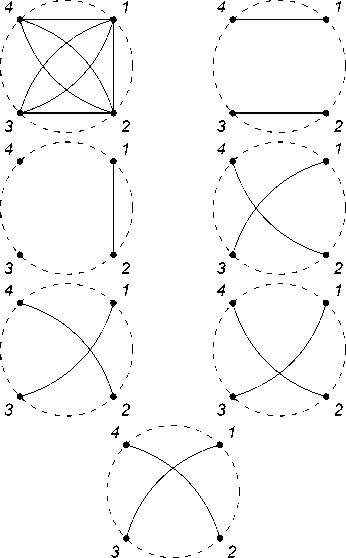
Fig. 8. The chord diagram G 2 (1 , 2 , 1) and its perfect matchings.

Рис. 8. Хордовая диаграмма G 2 (1 , 2 , 1) и ее совершенные паросочетания.

Let v _m denote the number of perfect matchings of G _m (1 , 2 , 1) . From (5) we get

V m = Hf( T 2 m (1 , 2 , 1)) =

m

= 2 m ^^

k =0

( — 1) ^{m -}k ( m + k _ 1) k !       ( m — k )!

By Proposition 2

v m ^∼

(2 m )! em m !

Taking v 1 = 1 and using (17) for consecutive m >  2 , we get the sequence A 336114 from [7]. This sequence is also presented in the second column of Table 2.

It is easy to see that sequences ( U _m ) and ( v _m ) are connected by the following relation:

v m — ^U m   ^U m- 1 •            ⁽¹⁸⁾

Indeed, thediagram G _m (1 , 2 , 2) differs from G _m (1 , 2 , 1) only by one edge joining the vertices 1 and 2 m . Hence, u m is greater than v m by the number of perfect matchings of G _m (1 , 2 , 2) , in which the vertices 1 and 2 m are joined by an edge, i.e., by u m- 1 . From equalities (16) and (18), one can derive the following recurrence relations for terms v _m :

V m +1 = (4 m + 3) V m - (4 m — 7) V m- 1 — V m- 2 , m >  4 . and

8 m ² V m + (2 m + 1) V m- 1     _ „

V m +1 = --------о----;-------- , m >  3 .

2 m - 1

• 2.6.    The arc diagram G m (1 , 2 , 0)

Let us consider the arc diagram G m (1 , 2 , 0) . Neighboring vertices are joined in it by one arc, the vertices 1 and 2 m are not adjacent if m >  2 , and all other pairs of vertices are joined by two arcs (see Fig. 9). Let w _m denote the number of perfect matchings of G m (1 , 2 , 0) . From (5) we get

Wm = Hf( T2 m (1, 2, 0)) = m     m-k-1

= E k=0

( m + k — 1)!

( m - k )!

( - 3 m + k )

Putting w 1 = 1 and using (19) for consecutive m >  2 , we get the sequence A 336286 from [7]. This sequence is also represented in the third column of Table 2. By

Proposition 2

w m ∼

(2 m )! em m !

It is not hard to see that sequences ( U _m ) and ( w _m ) are linked to each other by the following relationship:

W m = U m - 2 U m- 1 , m >  2 .       (20)

Indeed, the diagram G m (1 , 2 , 2) differs from G m (1 , 2 , 0) by two arcs joining the vertices 1 and 2 m . Hence, U _m is greater than w m by twice the number of perfect matchings of G m (1 , 2 , 2) , in which the vertices 1 and 2 m are joined by an arc, i.e., by 2 U _{m -} 1 . From equalities (16) and (20), we can derive the following recurrence relations for w _m with m >  4 :

Wm +1 = (4m + 4)Wm - (8m - 13)Wm-1 — 2Wm-2, and with m > 3:

W m +1 =

(32 m ² — 12 m + 2) W _m + (8 m + 1) W _{m -} 1 8 m — 7

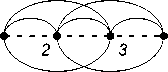
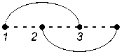
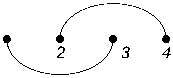
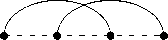
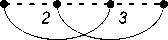
Fig. 9. The arc diagram G 2 (1 , 2 , 0) and its perfect matchings.

Рис. 9. Дуговая диаграмма G 2 (1 , 2 , 0) и ее совершенные паросочетания.

• 3. Conclusion

In this paper, we have considered the method for the explicit calculation of the hafnian of symmetric three-parameter Toeplitz matrices in polynomial time. In addition, in the case of non-negative integer parameters, this method allows us to calculate numbers of perfect matchings of various multigraphs represented in the form of arc and chord diagrams. Thus, we produce a certain class of integer sequences. Some sequences from this class have long been described in OEIS. But the method under consideration allows us to look at these sequences from the point of view of graph theory.