Hierarchical Pareto classification of the Russian regions by the population's quality of life indicators

Автор: Mironenkov Alexey A.

Журнал: Economic and Social Changes: Facts, Trends, Forecast @volnc-esc-en

Статья в выпуске: 2 т.13, 2020 года.

Бесплатный доступ

Improving population’s quality of life is a key goal of the state. In this regard, it is very important to correctly measure its level and, accordingly, classify the country’s regions by quality of life indicators. Most research in this area involves dividing variables into groups, unifying variables in each group and building an integral indicator, grouping or clustering objects as a linear convolution of variables with weights. Such approaches have their drawbacks due to the subjectivity of expert estimates, instability of the coefficients of the main component, inability to work with ordinal data, etc. Thus, the purpose of this study is to build a methodology for classifying the regions of the Russian Federation by quality of life indicators devoid of the above disadvantages. The proposed method is based on the concept of Pareto optimality well-known in Economics according to which all the regions are divided into disjoint classes. After dividing variables into groups we recommend using Pareto class as a representative of the category instead of the traditional unification and construction of intra-group convolutions, which is obtained after the intra-group Pareto classification, and building the final Pareto classification of the regions of the Russian Federation on the basis of the obtained intra-group Pareto classes. The advantage of the proposed approach is that it can be applied on the ordinal data, that is, when some variables are characterized only by their order and there are no exact values for each region. In addition, the algorithm is undemanding for computing power and does not use expert estimates, except for the selection of research variables. The main results of the study are the construction of a classification of the Russian Federation regions by quality of life indicators, comparison with traditional approaches and analysis of the features of the proposed methodology.

Еще

Regional ranking, population's quality of life indicators, stratification, pareto ratio, pareto dominance, pareto classification, pareto optimum, quality of life

Короткий адрес: https://sciup.org/147225448

IDR: 147225448 | DOI: 10.15838/esc.2020.2.68.11

Текст научной статьи Hierarchical Pareto classification of the Russian regions by the population's quality of life indicators

Ensuring high quality of life (QOL) of the country’s population is the central task of the state power institution in the vast majority of countries around the world. There is no single method for QOL measuring, and therefore there is no single mechanism for achieving the same “high QOL”. There is no doubt that this category includes many indicators that reflect various aspects of human life: economic indicators, indicators of the social sphere, access to public goods, the state of the environment, the level of security, and so on. In addition to the conditions that are common to the country’s entire population, the life of each individual is greatly affected by purely individual living conditions, such as the quality of health, marital status, and religious affiliation. In this regard, QOL is commonly referred to as a synthetic latent category.

As a rule, the general public estimates QOL in a given territory based on the GDP level or the related indicators (GNP, GRP per capita, etc.). However, the Easterlin paradox, described in 1974 [1], got us thinking about how plausible it is to measure QOL based on monetary indicators. Therefore, in order to explore the possibility of assessing economic results and social progress without relying on GDP indicators, a special Commission headed by J. Stiglitzand and A. Sen was created in 2008.

The Commission proposed three strategies for studying QOL. The first approach actually measures individual life satisfaction proposing to use the data from current surveys on how happy or satisfied individuals are with their lives. The second approach considers human life as an indivisible combination of various types of human activity and the personal freedom of choice of specific actions. The easier it is for a person to choose or do a specific action aimed at achieving his or her personal goals, the higher the QOL score is. The third approach involves weighing the QOL determinants for each individual or a group of individuals based on a subjective system of preferences. In other words, a certain list of human life spheres influencing the QOL is selected, and then either the individual is asked to independently assess the contribution of each of the proposed sphere, or the expert assigns a certain degree of influence on the QOL to the determinants. On the one hand, this approach avoids averaging the QOL assessment within the community, but, on the other hand, the mechanism of expert assessment cannot technically be unified for society as a whole.

There are two ways to track QOL indicators. The first is the construction of integral indicator (II) combining various aspects of human life that allow you to assess the success of the selected region, or community: the presence of a numeric expression QOL facilitates the territories ranging, makes it possible to compare them with each other, allows for a dynamic analysis. An alternative way to determine the level of QOL is to track a large number of wellbeing II simultaneously.

Today, we can talk about the “standard” method of calculating the QOL II: in the vast majority of studies, QOL is calculated as a linear convolution of a function, i.e.

f^x^1^, x(2),..., x(p)) = Tj=1ajx(j^ , (1) where x (^ is a statistical indicator, and Wj is the weight of the indicator determined by an expert way [2].

Similarly, the most cited QOL indicator, the Human Development Index (HDI) is calculated, which was developed by the UN in collaboration with A. Sen in 1990. HDI is a linear convolution of GNI by PPP per capita, life expectancy at birth and the level of education in the country.

Depending on the source of data which may be the results of a population survey or statistical collections, QOL indicators are usually divided into subjective (for example, Gallup-Healthways Global Well-Being index) and objective (already mentioned HDI), there are also indicators based on a combination of both approaches (Better Life Index).

The disadvantage of the “standard” method of QOL II calculating is the need to conduct an expert assessment of the indicators weight. And if when calculating the Better Life Index, the user assigns the contribution of the indicator (which, however, is already an II, and therefore it is formed using expert estimates of the indicators weight) to the final index, then the individuals are not involved in determining the calculation method for the rest of the indices. Thus, there will always be misrepresentation of information when moving from statistical data to the final II when calculating QOL II in this way.

Another method for QOL II calculating is described by S.A. Ayvazyan [3]. The author suggests reducing the number of model’ s regressors using the principal component method. The initial explanatory variables are divided into blocks that characterize one area of human life: the quality of the population, the welfare (standard of living) of the population, social security (quality of the social sphere), the quality of the environment (ecological niche), and natural and climatic conditions. Then, there are two ways depending on the features of the model, either the II is calculated using the main components method separately for each block, and then the block II are combined into a final single index; or the main component is immediately found for all regressors simultaneously, then it becomes the final II QOL. The advantages of the method are the exclusion of expert evaluation of weights determining, ease of use and relative ease of calculation.

The method proposed by S.A. Ayvazyan is criticized because of the instability of determining weight coefficients, which is explained by the peculiarities of calculating the main components and cannot be corrected using standard statistical data processing packages [4].

The disadvantages associated with building a single II QOL can be overcome by using an alternative approach of simultaneously tracking a large number of well-being II. Its followers note that when information is rolled up into a single indicator, first, there is always a distortion and/or loss of information, and second, there are always difficulties in determining the share of indicators’ contribution to the final II. Some countries have successfully implemented the programs of improving the population’s QOL by tracking individual indicators: in Australia it is Measures of Australia’s Progress, in the UK it is Measuring National Well-being program, in New Zealand it is The Quality of Life Project, etc. The projects involve tracking more than 40 indicators, the composition and number of which can be either unchanged (as in the case of New Zealand since 1999) or changing (in the UK, 41 indicators were estimated in 2015, and 43 in 2016). It is obvious that QOL assessment is devoid of researchers’ subjective contribution within this approach [5], but the complexity of the process, as well as the inability to assess the progress of social and economic development of the territory over time, make it less attractive to the general public.

In order to achieve the main purpose of the research, i.e. ranking Russian subjects by QOL level, we propose a method of QOL analysis that, first, is devoid of the researcher’s subjective intervention, second, allows comparing the regions with each other even by ordinal data, and third, would be technically easy to implement.

Russian regions today are highly differentiated by all indicators, macro-economic and micro-economic ones; however, there is no doubt that some constituent entities, such as Moscow, Saint Petersburg, and the Krasnodar Krai, are the territories with a higher QOL level. This is evidenced, on the one hand, by the direction of internal migration flows [6], and on the other hand, by the high level of real estate prices [7]. Therefore, we propose to divide the constituent entities into classes, identifying the leading and outsider regions in terms of QOL indicators, and then analyze these classes, which can help the Institute of state power in finding the methods to increase the QOL level.

Multi-criteria classification methods

Quite often, in practice, there is a need to classify the sample according to many criteria simultaneously, for example, when selecting reliable banks or companies with high investment potential.

The multi-criteria classification task can be formulated as follows. Suppose there are N objects each having P characteristics. After completing the task, we will get K classes (where K is not known in advance), each of them contains objects that are as close to each other as possible by all P characteristics.

The vast majority of methods that can be used for multi-criteria classification require the researcher’s intervention: the method helps to rank objects by their attractiveness or success rate. Then they should be divided into classes according to the II value in an expert way. To solve this problem, the following methods can be used:

• K-means method and its modifications

The method is based on the assumption of geometric proximity of objects to each other in the P-dimensional space of descriptive indicators. When using the method, to identify the optimal number of classes, a certain optimality criterion is needed that sets the distance between the cluster centers. The method is used to identify high-risk countries [8].

• Ranking the sample by the index value based on linear convolution

A system of weights of characteristics in the final index should be put in to implement this method. Then the array of source objects ranked by the index value can be divided into classes in an expert way. II option constructed using the principal component method was used in [9] to classify countries by the level of social comfort of the population.

• Ranking by influence

Researchers San, Han, Zhao, and others [10] proposed an algorithm for rating authors of scientific papers. The essence of the method is as follows: the more important variables are highlighted among all the explanatory ones. A higher rank is assigned to the objects with a high value of more important criteria. Then all explanatory variables for high-ranked objects are analyzed: the greater the contribution of the criterion to the high-ranked object is, the higher the weight of this criterion is throughout the system.

• Ranking according to the Borda rule

The method was used to analyze the performance of regional bank branches [11]. Objects are ranked separately for each of the criteria, and the final rank is obtained by simply summing the ranks for each criterion.

• Classification based on linear optimization of weights

The method is often used to divide the company’s raw materials by the degree of importance in inventory management [12; 13]. First, the linear programming problem is solved sequentially for each object relative to the weights, and then the objects under consideration are ranked based on the resulting weight vector.

• Linstrat method

Stratification occurs by combining the neighboring objects projections on a hyperplane defined by weights of criteria. The implementation of the method based on the data of bibliometric indicators of journals and countries is proposed [14].

• Pareto Classification

There are non-dominated objects grouped into a single class at each step of the algorithm in the original sample. At the next step, the objects are excluded from consideration, and the procedure is repeated for the remaining objects. The method is well known for a long time [15; 16; 17]. It is possible to specify the works considering the Pareto ratio as an object [18; 19], but it is used relatively rarely when studying the quality of life [20; 21].

We will use Pareto classification n the research.

Pareto classification

Suppose there are two regions, a and b, each having a characteristic vector x“ and x^, where i = 1, _, p is responsible for the feature number; in total, p features are considered in each region. Let’s say that object a is Pareto dominant over object b if two conditions are met simultaneously:

1. Vi: x f > x f ,
2. 3i: x “ > x f .

In other words, region a is Pareto dominant over region b if region a is no worse than region b by all the considered features, and there is at least one feature where region a is strictly superior to region b. We should that the Pareto dominance ratio may not exist between two randomly selected objects.

Suppose there are n objects (regions), each having a feature vector x. Let’s call object a Pareto optimal if there is no object dominating a among the objects in the sample. By checking each region for Pareto dominance, we get a subset of Pareto-optimal regions. Let’s call this subset the first Pareto class. In other words, a region is included in the first Pareto class if it is impossible to specify another region that is not worse by all its indicators than the one under consideration, and is strictly better by at least one of the indicators.

Excluding the regions of the first Pareto class and selecting the Pareto-optimal regions from the remaining ones, we get a subset of the regions that form the second Pareto class. We perform this procedure until unclassified regions remain in the sample. Thus, as a result, the original set of regions is represented as a sequence of disjoint non-empty subsets. In this case, for each region from a lower (with a higher number) class, there is at least one region from a higher Pareto class that is Pareto-dominated.

We should emphasize that it is impossible to predict the number of Pareto classes obtained in advance. So, when all pairwise rank correlation coefficients are close to unity, the division into Pareto classes is very fractional, and the number of classes is close to the number of regions. In the reverse degenerate case, when there is at least one pairwise rank correlation coefficient close to minus unity, the number of Pareto classes is small; it is quite possible that all regions will be assigned to a single first class. In practice, the latter situation is not possible in the problems of quality of life research, since the more the variables used are ordered “the better the quality of life is”, which determines a direct rank relationship between the variables and a rank correlation coefficient that is obviously different from minus unity.

Research methodology

Let’s highlight the main stages of the research:

• data collection;
• formation of a posteriori set of the grouped partial criteria;
• logical unification;
• Pareto classification of the regions within the groups;
• Pareto classification of the classes in all

groups.

The formation of a posteriori set of partial criteria is based on the selection of a list of partial indicators x ⁽¹⁾ ,x ⁽²⁾ , .„, x ^(p) , which are obtained from the original a priori (theoretical) list of statistical indicators x ⁽¹⁾ , x ⁽²⁾ , .„, x ^(k) , provided к >p . This set of indicators should sufficiently characterize the analyzed synthetic category of quality of life. The variables that characterize similar aspects are grouped together. The selected indicators are called private criteria, and the set of the grouped selected indicators of quality of life is called a posteriori set of private criteria [2].

Logical unification means bringing all data in a comparable form.

This transformation will allow to:

• get rid of the influence of the region size on the criteria value;
• rank the criteria values by relative, rather than absolute, characteristics;
• compare the regions with each other regardless of the regions’ size.

The next step of unification is widespread [2; 9]. It consists in switching to [0; N] – point scales in measuring particular quality of life criteria. The value 0 corresponds to the lowest quality of life, and N – to the highest. Within the framework of this research, the value of N is 10.

If a particular criterion x is associated by a monotonically increasing dependence with the integral property of life quality (i.e., the higher the value of x , the higher its quality value), then the unified variable is calculated by the following formula:

^xi = x ZZ ^— * ^ , (2)

лтах лтт where xmin is the smallest value of the original indicator (the worst);

x_max is the highest value of the original indicator (the best).

If a particular criterion x is connected by a monotonically decreasing dependence with an integral property of life quality (the higher the value of x , the lower its quality value), then the unified variable is calculated as follows:

-, where xmin is the smallest value of the original indicator (the worst);

x_max is the highest value of the original indicator (the best).

We should note that the result of Pareto classification will not change if, instead of the generally accepted unification procedure described above, we restrict ourselves to ranks with ascending sorting for variables having a positive impact on the quality of life, and descending ordering for the rest.

Next, a Pareto classification is performed for a set of variables within each group. As a result, each region gets the class number it belongs to within this group of variables.

Then a Pareto classification is performed based on the results obtained, which makes it possible to obtain Pareto classes of regions based on their intra-group Pareto classes.

Research information support

The empirical part of the research is based on the data from the statistical digest “Regions of Russia. Socio-economic indicators. 2016”. The digest contains information on the development of industries and sectors of the economy for the period of 2005–2016 for the subjects of the Russian Federation:

• employment;
• level of welfare and economic status of the population;
• ecological situation;
• development of the social security system;
• state of small business;
• dynamics of price levels in the consumer and manufacturing sectors.

In addition, we used the information from the digest “Regions of Russia. Main characteristics of the subjects of the Russian Federation”.

Based on the above analysis of QOL indicators in accordance with the requirements advanced by S.A. Ayvazyan in the monograph [2, p. 78] on (a) relevance, (b) information availability and (c) reliability of information, we have chosen 33 private indicators organized in five basic groups of synthetic categories characterizing the population’s activity in the regions.

1. Socio-demographic indicators : migration growth, total mortality rates, life expectancy at birth, migration growth rates, labor force, number of registered crimes.
2. Economic and financial indicators : per capita income of the population; gross regional product (GRP); retail trade turnover, wholesale trade turnover; investment in fixed assets; turnover of organizations; cost of fixed assets.
3. Infrastructure indicators : departure of passengers by bus; density of paved public roads; number of hospital beds; stadiums with stands for 1,500 seats or more; flat sports facilities; gyms; swimming pools; quantity of professional educational organizations training middle-level specialists; quantity of higher education organizations; tourist companies; commissioning of apartments; quantity of organizations performing research and development.
4. Environmental indicators : emissions of pollutants from stationary sources into the air; capture of air pollutants from stationary sources; use of fresh water.
5. Production indicators : number of enterprises and organizations; mining; manufacturing; production and distribution of electricity, gas and water; volume of construction work.

The result of Pareto classification of the Russian regions (empirical results of the study)

According to the results of the intragroup Pareto classifications, the regions of the Russian Federation were stratified into the following number of classes in each group of variables:

1. Socio-demographic indicators: 5 Pareto classes.
2. Economic and financial indicators: 11 Pareto classes.
3. Infrastructure indicators: 7 Pareto classes.
4. Environmental indicators: 10 Pareto classes.
5. Production indicators: 9 Pareto classes.

In the supergroup Pareto classification, the regions were divided into 10 classes based on their comparison by the intragroup classes. Detailed stratification results for each region considered are shown in table 1.

Table 1. Pareto classes of the regions of the Russian Federation by groups of variables and the final Pareto class

RF Region	Intragroup Pareto classes					Pareto class of the region
RF Region	Sociodemographic indicators	Economic and financial indicators	Infrastructure indicators	Environmental indicators	Production indicators	Pareto class of the region
Tyumen Oblast	1	1	1	1	1	1
Moscow	1	1	1	3	1	2
Krasnodar Krai	1	3	1	2	2	2
Leningrad Oblast	1	5	2	1	4	2
Republic of Dagestan	1	5	2	1	4	2
Stavropol Krai	1	5	2	1	4	2
Kabardino-Balkar Republic	1	9	3	2	8	3
Moscow Oblast	1	2	1	3	2	3
Republic of Ingushetia	1	11	3	1	9	3
Rostov Oblast	2	4	1	2	3	3
Chukotka Autonomous Okrug	3	1	5	5	8	3
Astrakhan Oblast	3	7	5	2	6	4
Saint Petersburg	1	2	2	4	2	4
Sevastopol	1	10	3	2	8	4
Krasnoyarsk Krai	2	4	2	3	2	4
Perm Krai	4	4	3	2	3	4
Republic of Bashkortostan	2	4	1	6	3	4
Republic of Kalmykia	3	11	6	1	9	4
Republic of Tatarstan	2	3	1	7	2	4
Sverdlovsk Oblast	2	3	1	7	2	4
Chechen Republic	1	9	3	3	7	4
Belgorod Oblast	1	5	2	6	4	5
Voronezh Oblast	2	4	2	4	4	5
Kamchatka Krai	2	3	6	4	7	5
Kemerovo Oblast	4	5	2	4	2	5
Kostroma Oblast	4	9	4	2	7	5
Murmansk Oblast	3	3	5	4	4	5
Nizhny Novgorod Oblast	2	4	2	5	3	5
Orenburg Oblast	3	5	3	4	3	5
Republic of Adygea	1	9	3	3	8	5
Republic Of Sakha (Yakutia)	2	3	4	8	3	5
Republic of North Ossetia	2	10	2	3	7	5
Sakhalin Oblast	4	2	6	5	2	5
Tver Oblast	4	7	3	3	5	5
Khabarovsk Krai	4	3	4	5	4	5
Kursk Oblast	2	7	2	4	5	6
Magadan Oblast	4	2	7	6	7	6
Novosibirsk Oblast	2	5	2	7	3	6
Oryol Oblast	4	8	3	3	8	6
Republic of Altay	2	11	6	3	9	6
Republic of Crimea	2	6	2	4	6	6
Samara Oblast	3	4	2	6	3	6
Saratov Oblast	2	6	3	5	4	6
Tula Oblast	1	6	2	6	5	6
Udmurt Republic	3	6	3	4	4	6
Chelyabinsk Oblast	2	4	2	8	3	6

End of table 1

Let us enlarge on the Pareto classification process directly. We should note that, for example, in the group of “Financial and economic indicators” containing seven indicators, exactly three regions are assigned to the first class. That is, each of these regions did not find another one that was not worse (and in some ways better) by

these seven variables. If these three regions are not taken into account, then the other subjects have four more regions that can be called “the best of the remaining”, i.e. the second Pareto class for this group is formed by four regions. Similarly, an intragroup classification is constructed for each group of variables.

RF Region	Intragroup Pareto classes					Pareto class of the region
RF Region	Sociodemographic indicators	Economic and financial indicators	Infrastructure indicators	Environmental indicators	Production indicators	Pareto class of the region
Altai Krai	3	6	2	7	5	7
Arkhangelsk Oblast	3	4	4	7	4	7
Vladimir Oblast	3	7	2	4	5	7
Irkutsk Oblast	3	5	3	6	3	7
Kaliningrad Oblast	2	7	3	4	5	7
Kaluga Oblast	2	7	2	5	5	7
Lipetsk Oblast	2	6	2	9	5	7
Omsk Oblast	3	5	2	8	4	7
Primorsky Krai	3	4	4	7	4	7
Republic of Komi	4	4	5	7	3	7
Ryazan Oblast	1	7	3	7	6	7
Tomsk Oblast	2	6	4	7	5	7
Yaroslavl Oblast	3	6	3	5	5	7
Bryansk Oblast	4	7	2	8	7	8
Volgograd Oblast	3	5	3	6	4	8
Penza Oblast	2	7	3	5	6	8
Republic of Mari El Republic	2	9	4	4	7	8
Smolensk Oblast	3	7	3	5	5	8
Chuvash Republic	2	8	2	5	6	8
Amur Oblast	5	5	5	10	4	9
Vologda Oblast	4	5	4	8	5	9
Jewish Autonomous region	5	9	6	4	9	9
Ivanovo Oblast	3	8	2	6	7	9
Karachay-Cherkess Republic	2	10	4	4	8	9
Kirov Oblast	4	7	4	6	6	9
Pskov Oblast	3	9	4	5	7	9
Republic of Buryatia	2	8	5	5	6	9
Republic of Mordovia	2	8	3	7	7	9
Tambov Oblast	3	6	3	7	7	9
Ulyanovsk Oblast	3	7	3	7	5	9
Zabaykalsky Krai	4	8	5	6	6	10
Kurgan Oblast	5	8	4	7	7	10
Novgorod Oblast	4	8	4	8	5	10
Republic of Karelia	4	8	5	6	6	10
Republic of Tyva	3	11	6	4	8	10
Republic of Khakassia	3	9	5	9	6	10

Table 2. Results of various classifications of the Russian Federation regions

RF Regions	Pareto	B.M. Grinchel		A.O. Polynev		RIA Rating
RF Regions	class (out of 10)	rating value	rank (out of 80)	rating value	rank (out of 80)	rating value	rank (out of 80)
Altai Krai	7	6.8	60	6.8	62	6.9	68
Amurskaya Oblast	9	6.8	58	6.8	62	6.3	49
Arkhangelsk Oblast	7	7.8	73	6.5	52	7.1	70
Astrakhan Oblast	4	5.2	15	6.1	35	6.5	52
Belgorod Oblast	5	4.2	4	4.4	4	4.3	5
Bryansk Oblast	8	6.2	42	6.7	57	6.2	46
Vladimir Oblast	7	6.8	57	6.3	44	6.0	31
Volgograd Oblast	8	6.3	44	6.2	37	6.0	34
Vologda Oblast	9	7.9	75	6.7	57	6.7	58
Voronezh Oblast	5	4.6	6	5.8	26	4.7	7
Moscow	2	2.2	2	2.3	1	3.1	1
Saint Petersburg	4	2.1	1	3.0	2	3.2	2
Jewish Autonomous Region	9	8.1	79	7.1	70	7.7	73
Zabaykalskiy Krai	10	7.4	70	7.2	72	8.0	78
Ivanovo Oblast	9	6.4	49	6.4	48	6.2	45

1 RIA Rating. The rating of the Russian regions by quality of life in 2018. Available at:

Continuation of table 2

RF Regions	Pareto	B.M. Grinchel		A.O. Polynev		RIA Rating
RF Regions	class (out of 10)	rating value	rank (out of 80)	rating value	rank (out of 80)	rating value	rank (out of 80)
Irkutsk Oblast	7	7.9	77	6.6	56	6.8	63
Kabardino-Balkarian Republic	3	6.0	34	6.8	62	7.3	71
Kaliningrad Oblast	7	5.2	15	5.2	10	4.9	9
Kaluga Oblast	7	5.1	11	5.5	17	5.4	18
Kamchatka Krai	5	6.1	37	5.7	24	6.0	29
Karachay-Cherkess Republic	9	7.9	76	8.4	79	8.1	79
Kemerovo Oblast	5	8.0	78	5.8	28	6.4	50
Kirov Oblast	9	7.1	63	6.9	68	6.7	59
Kostroma Oblast	5	6.5	52	6.9	66	6.7	56
Krasnodar Krai	2	5.7	31	5.1	8	4.4	6
Krasnoyarsk Oblast	4	7.1	64	5.5	17	6.1	42
Kurgan Oblast	10	7.7	72	7.4	75	7.8	74
Kursk Oblast	6	4.8	8	5.6	20	5.2	13
Leningrad Oblast	2	6.5	50	5.2	12	5.0	10
Lipetsk Oblast	7	5.2	17	5.4	15	4.8	8
Magadan Oblast	6	5.6	23	5.5	19	6.0	32
Moscow Oblast	3	4.3	5	4.1	3	3.6	3
Murmansk Oblast	5	6.1	39	5.8	26	6.0	33
Nizhegorod Oblast	5	5.2	14	5.6	20	5.3	14
Novgorod Oblast	10	6.9	61	5.8	28	6.7	57
Novosibirsk Oblast	6	5.1	12	5.3	13	5.6	21
Omsk Oblast	7	5.6	23	6.2	37	6.6	53
Orenburg Oblast	5	6.6	53	6.3	44	6.0	30
Oryol Oblast	6	5.8	33	6.4	48	6.0	38
Penza Oblast	8	5.6	28	6.4	51	5.9	27
Perm Krai	4	6.4	48	6.2	37	6.1	39
Primorski Krai	7	7.0	62	6.6	54	6.2	47
Pskov Oblast	9	7.4	68	6.6	54	6.6	54
Republic of Adygea	5	6.5	51	5.9	32	5.9	28
Altai Republic	6	7.8	74	6.2	37	7.8	75
Republic of Bashkortostan	4	5.6	27	5.2	10	5.7	22
Republic of Buryatia	9	7.4	66	7.2	72	7.6	72
Republic of Dagestan	2	5.5	21	7.2	71	6.8	64
Republic of Ingushetia	3	5.6	23	7.6	76	7.8	77
Republic of Kalmykia	4	7.4	67	8.5	80	7.8	76
Republic of Karelia	10	7.4	69	6.2	37	7.1	69
Komi Republic	7	7.6	71	6.4	48	6.7	60
Mari El Republic	8	6.6	56	7.3	74	6.8	62
Republic of Mordovia	9	6.0	35	6.9	68	6.1	41
Republic of Sakha (Yakutia)	5	6.6	54	6.8	62	6.9	67
Republic of North Ossetia – Alania	5	4.7	7	6.2	37	6.7	61
Republic of Tatarstan	4	4.2	3	4.5	5	4.2	4
Tyva Republic	10	8.6	80	8.3	78	9.0	80
Republic of Khakassia	10	7.1	64	6.9	66	6.5	51
Rostov Oblast	3	6.2	40	6.1	33	5.3	17
Ryazan Oblast	7	5.7	29	6.1	33	5.8	23
Samara Oblast	6	5.6	22	5.0	7	5.3	16
Saratov Oblast	6	5.3	19	5.8	28	6.0	35
Sakhalin Oblast	5	5.3	20	5.6	20	6.1	43

End of table 2

RF Regions	Pareto	B.M. Grinchel		A.O. Polynev		RIA Rating
RF Regions	class (out of 10)	rating value	rank (out of 80)	rating value	rank (out of 80)	rating value	rank (out of 80)
Sverdlovsk Oblast	4	5.6	26	4.7	6	5.1	11
Smolensk Oblast	8	6.4	47	6.3	44	6.0	36
Stavropol Krai	2	5.8	32	5.8	28	5.5	19
Tambov Oblast	9	4.9	10	6.1	35	6.0	37
Tver Oblast	5	6.1	38	6.3	44	6.6	55
Tomsk Oblast	7	6.1	36	5.4	15	6.3	48
Tula Oblast	6	6.2	41	5.7	24	5.3	15
Tyumen Oblast	1	4.9	9	5.1	8	5.1	12
Udmurt Republic	6	6.3	43	6.7	57	6.1	40
Ulyanovsk Oblast	9	6.4	46	6.7	57	5.9	25
Khabarovsk Krai	5	6.3	45	6.2	37	5.9	26
Chelyabinsk Oblast	6	6.8	59	5.3	13	5.5	20
Chechen Republic	4	6.6	55	8.0	77	6.8	66
Chuvash Republic	8	5.2	17	6.7	57	6.1	44
Chukotka Autonomous Okrug	3	5.1	13	6.5	52	6.8	65
Yaroslavl Oblast	7	5.7	30	5.6	20	5.8	24

As can be seen from table 1, the final Pareto classification divided the subjects into ten classes on the basis of the intra-group classifications results. The first Pareto class which is the highest one, includes only one region, the Tyumen Oblast. It was assigned to the first class in all groups of variables. The second class consists of five regions: Moscow, Krasnodar Krai, Stavropol Krai, Leningrad Oblast, and the Republic of Dagestan. The third class also includes five regions: the Moscow and Rostov Oblasts, the Kabardino-Balkar Republic, the Republic of Ingushetia, and the Chukotka Autonomous Okrug. Classes four through ten consist, respectively, of 10, 14, 11, 13, 6, 11, 6 regions.

Results discussion

We should note, that the results generally correlate well with the regions classifications known to the author, taking into account a radically different ranking method. Thus, the subjects that are traditionally classified as leading regions are located in the upper classes

in the case of Pareto ranking, while those that are usually classified as depressed, i.e. outsider regions, occupy mainly the last classes.

Let us compare the results obtained with the results of the works known to the author. B.M. Grinchel and E.A. Nazarova give generalized point estimates of the quality of life in the regions of Russia [22, p. 118]. In the study of the Ministry of economic development [23], A.O. Polynev, I.V. Grishina, and S.A. Timonin use S.A. Ayvazyan’s methodology applied to later data to calculate QOL indicators. Finally, in February 2019, RIA Rating Agency released a rating of Russian regions on the quality of life of the population¹. The ratings are based on various methods based on the data on the Russian regions’ socio-economic state for the period of 2014-2018. However, not all studies coincide in a set of regions, for example, the earlier ones do not have data on the Republic of Crimea and the city of Sevastopol. The classification results are summarized in table 2 .

The correlation matrix shows a very high consistency between the ratings of the Russian regions calculated according to the traditional methods ( Table 3 ).

Table 3. Correlation matrix

		CD S CD	О	cc
Pareto class	1
B.M. Grinchel	-0.51	1
A.O. Polynev	-0.44	0.72	1
RIA Rating	-0.46	0.78	0.88	1

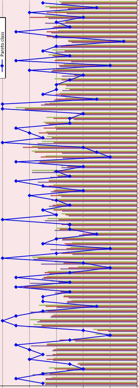
The result of Pareto classification is slightly different from them. The correlation coefficient negative sign is easily explained: the smaller the Pareto class, the higher the quality of life index. Let us look at the differences in more detail. Since the results are obtained in different scales, we will bring the rating results to comparable values by linear shift, for perception convenience² ( Figure ).

It is apparent that having a very good consistency between the ratings evaluated by the generally accepted methodology, the Pareto classification generally agrees with them in terms of dynamics, and similar results were obtained for the vast majority of the regions.

However, the Pareto classification also led to uncharacteristic results. Thus, Moscow and the Tyumen Oblast, traditionally considered to be the leading regions, are located in different classes. The Tyumen Oblast outperforms the capital in terms of environmental indicators, but they are identical by other indicators. In this regard, the Tyumen Oblast fell into a higher Pareto class. Similarly, the difference between the Pareto classes of the Republic of Dagestan and the Republic of Ingushetia is explained. Despite the equality of results in the groups of “Socio-demographic indicators” and “Environmental indicators” and a slight (in absolute terms) superiority in other groups of variables there is a Pareto ratio between the

Values of the Pareto-class and the given ratings according to the standard methods

Yaroslavl Oblast

Chukotka Autonomous Okrug Chuvash Republic

Chechen Republic Chelyabinsk Oblast Khabarovsk Krai Ulyanovsk Oblast Udmurt Republic Tyumen Oblast Tula Oblast

Tomsk Oblast Tver Oblast Tambov Oblast Stavropol Krai Smolensk Oblast Sverdlovsk Oblast Sakhalin Oblast

Saratov Oblast Samara Oblast Ryazan Oblast Rostov Oblast

Republic of Khakassia

Tyva Republic

Republic of Tatarstan

Republic of North Ossetia - Alania Republic of Sakha (Yakutia)

Republic of Mordovia

Mari El Republic Komi Republic Republic of Karelia Republic of Kalmykia Republic of Ingushetia Republic of Dagestan Republic of Buryatia

Republic of Bashkortostan Altai Republic

Republic of Adygea Pskov Oblast

Primorski Krai

Perm Krai

Penza Oblast

Oryol Oblast

Orenburg Oblast Omsk Oblast

Novosibirsk Oblast Novgorod Oblast

Nizhny Novgorod Oblast Murmansk Oblast

Moscow Oblast Magadan Oblast

Lipetsk Oblast Leningrad Oblast Kursk Oblast

Kurgan Oblast

Krasnoyarsk Oblast Krasnodar Krai Kostroma Oblast Kirov Oblast

Kemerovo Oblast

Karachay-Cherkess Republic Kamchatka Krai

Kaluga Oblast

Kaliningrad Oblast Kabardino-Balkarian Republic Irkutsk Oblast

Ivanovo Oblast Zabaykalskiy Krai

Jewish Autonomous Region Saint Petersburg Moscow

Voronezh Oblast

Vologda Oblast Volgograd Oblast Vladimir Oblast Bryansk Oblast Belgorod Oblast Astrakhan Oblast

Arkhangelsk Oblast Amurskaya Oblast Altai Krai

The vertical columns present the values of the regions’ ratings evaluated as linear convolutions. Polyline shows the results of classification of the Russian Federation regions based on the Pareto ratio.

republics determining the difference in the classes of regions. The Caucasian republics of Dagestan, Ingushetia, and Kabardino-Balkaria took a relatively high place in the rating: having a high class in the groups of “Sociodemographic variables” and “Environmental variables”, they have only one or two levels of Pareto-dominant regions.

The practical significance of the research consists in the possibility of using Pareto classification algorithms as a way to work with ordinal data, as well as a way to obtain numerical characteristics in a situation where only the order relation is known by some features. The classification approach based on the Pareto ratio can also be used in making management decisions, since, unlike, for example, neural networks, not only the result is known, but also the information about the causes of this class is stored, in particular, which group of variables contributed to getting into a lower

class and, accordingly, which area should be given additional attention.

To sum up, we can conclude that, despite a fundamentally different approach applied, the results of Pareto classification of the Russian regions are generally consistent with the results of traditional ratings, and they have undeniable advantages. Thus, the proposed method is able to work successfully with the data measured in ordinal scales (i.e., only considering the information about who is better in each pair by the selected indicator), without using absolute values. The main operation used is binary multiplication, so the algorithm execution speed is high enough even in case of outdated computers. We should also note that Pareto classification is not a common method, its algorithm does not have a built-in implementation in any of the data processing packages known to the author, which in turn prevents its wide distribution.

Список литературы Hierarchical Pareto classification of the Russian regions by the population's quality of life indicators

Easterlin R.A. Does Economic growth improve the human lot? Some empirical evidence. In: P.A. David, M.W. Reder. Nations and Households in Economic Growth: Essays in Honor of Moses Abramowitz. N.Y.: Academic Press, 1974, рр. 89–125. Available at: https://doi.org/10.1016/B978-0-12-205050-3.50008-7
Aivazyan S.A. Analiz kachestva i obraza zhizni naseleniya [Analysis of the Quality of Life and the Lifestyle of the Population]. Moscow: Nauka, 2012. 432 p.
Aivazyan S.A. Russia in cross-national analysis of synthetic categories of the quality of population life. Part 1. Analysis Methodology and Example of its Implementation. Mir Rossii. Sotsiologiya. Etnologiya=Universe of Russia, 2001, no. 4, pp. 59–96. (in Russian)
Zhgun T.V. Building an integral measure of the quality of life of constituent entities of the russian federation using the principal component analysis. Ekonomicheskie i sotsial’nye peremeny: fakty, tendentsii, prognoz=Economic and Social Changes: Facts, Trends, Forecast, 2017, vol. 10, no. 2, pp. 214–235. DOI: 10.15838/esc.2017.2.50.12 (in Russian)
Kislitsyna O.A. Izmereniya kachestva zhizni/blagopoluchiya: mezhdunarodnyi opyt [Measurement of the Quality of Life / Well-Being: International Experience]. Moscow: Institut ekonomiki RAN, 2016. 62 p. ISBN 978-5-9940-0541-5
Mkrtchyan N.V., Karachurina L.B. Migration in Russia: flows and centers of attraction. Demoskop Weekly=Demoskop Weekly, 2014, no. 595–596. Available at: http://www.demoscope.ru/weekly/2014/0595/tema01.php (in Russian)
Mints V. On factors of housing prices dynamics. Voprosy ekonomiki=Voprosy Ekonomiki, 2007, no. 2, pp. 111–121. (in Russian)
Smet Yves De, Linett Montano Guzmán. Towards multicriteria clustering: An extension of the k-means algorithm. European Journal of Operational Research, 2004, no. 158 (2), pp. 390–398. Available at: https://doi.org/10.1016/j.ejor.2003.06.012
Leshchaykina M.V. Econometric cross-country analysis of the living population social comfort. Prikladnaya ekonometrika=Applied Econometrics, 2014, no. 36 (4). Pp. 102–117. (in Russian)
Sun Y., Han Jiawei, Zhao Peixiang, Yin Zhijun, Cheng Hong, Wu Tianyi. RankClus: integrating clustering with ranking for heterogeneous information network analysis. Proceedings of the 12th International Conference on Extending Database Technology: Advances in Database Technology, 2009, pр. 565–576.
Aleskerov F., Ersel H., Yolalan R. Multicriterial ranking approach for evaluatingbank branch performance. International Journal of Information Technology & Decision Making, 2004, vol. 3, no. 2, рр. 321–335. Available at: https://doi.org/10.1142/S021962200400101X
Ramanathan R. ABC inventory classification with multiple-criteria using weighted linear optimization. Computers & Operations Research, 2006, vol. 33, no. 3, рр. 695–700. Available at: https://doi.org/10.1016/j.cor.2004.07.014
Douissa M.R., Jabeur K. A New model for multi-criteria ABC inventory classification: PROAFTN method. Procedia Computer Science, 2016, no. 96, pp. 550–559. Available at: https://doi.org/10.1016/j.procs.2016.08.233
Orlov M.A. An algorithm for multicriteria stratification. Biznes-informatika=Business Informatics, 2014, no. 4 (30), pp. 24–35. (in Russian)
Buchanan J.M. The relevance of Pareto optimality. Journal of conflict resolution, 1962, vol. 6, no. 4, pp. 341–354.
Rodríguez J.D., Lozano J.A. Multi-objective learning of multi-dimensional Bayesian classifiers. Eighth International Conference on Hybrid Intelligent Systems, 2008, рр. 501–506. DOI: 10.1109/HIS.2008.143
Satchidananda Dehuri, Sung Bae Cho. Multi-objective classification rule mining using gene expression programming. 2008 Third International Conference on Convergence and Hybrid Information Technology. Busan, 2008, pp. 754–760. DOI: 10.1109/ICCIT.2008.27
Talukder A.K.M., Deb K., Blank J. Visualization of the boundary solutions of high dimensional pareto front from a decision maker’s perspective. Proceedings of the Genetic and Evolutionary Computation Conference Companion, 2018, July, pp. 201–202. DOI: 10.1145/3205651.3205782
Désilles A., Zidani H. Pareto front characterization for multiobjective optimal control problems using Hamilton-Jacobi approach. SIAM Journal on Control and Optimization, 2019, no. 57(6), рр. 3884–3910. doi.org/10.1137/18M1176993.
Shakin V.V. Pareto classification of the finite sample sets, applications of multivariate statistical analysis in economics and assessment of production quality. Proceedings of V Scientific Conference of CIS States, RAS CEMI, 1993.
Kolenikov S. The Methods of the Quality of Life Assessment. NES, 1999.
Grinchel’ B.M., Nazarova E.A. Typology of regions by level and dynamics of the quality of life. Ekonomicheskie i sotsial’nye peremeny: fakty, tendentsii, prognoz=Economic and Social Changes: Facts, Trends, Forecast, 2015, no. 3, pp. 111–125. DOI: 10.15838/esc/2015.3.39.9 (in Russian)
Polynev A.O., Grishina I.V., Timonin S.A. Quality of life of Russian regions’ population: Research methodology and results of comprehensive evaluation. Sovremennye proizvoditel’nye sily. Ot dogonyayushchego k operezhayushchemu razvitiyu=Modern Productive Forces. From Catching-up Development to Advanced Development, 2012., no. 1, pp. 70–84. (in Russian)

Еще

Статья научная