High-speed Image compression based on the Combination of Modified Self organizing Maps and Back-Propagation Neural Networks

Published Online April 2014 in MECS DOI: 10.5815/ijigsp.2014.05.04

The main advantage of compression is that it reduces the data storage requirements. It also offers an attractive approach to reduce the communication cost in transmitting high volumes of data over long-haul links via higher effective utilization of the available bandwidth in the data links. This significantly aids in reducing the cost of communication due to the data rate reduction. Because of the data rate reduction, data compression also increases the quality of multimedia presentations through limited-bandwidth communication channels [1]. Image compression is one of the important challenges in the information compression on the other hand artificial neural networks have become popular over the last ten years for diverse applications for image compression to machine vision and image processing.

High performance image compression algorithms may be developed and implemented in those neural networks. The neural network image compression algorithm can be summarized as follows:

• 1-    Back-Proagation image compression

• 2-    Hebbian learning based image compression

• 3-    Vector Quantization (VQ) neural networks.

• 4-    Predictive neural networks.

In this paper the proposed method is based on two major stages, the first stage is MSOFM and the second stage is back-propagation algorithm. In the first stage by MSOFM and the proposed weight update method estimated a distribute function of the input image in lower dimensions by neurons (weight matrix) this is first data compression. In second stage weight matrix is applied to back-propagation algorithm until another stage of compression is applied to the input image. Figure 1 shows a block diagram of the proposed method.

Estimated Image On Neurons

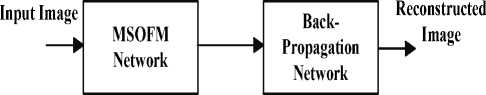
Figure 1. Block diagram of the proposed method.

As seen in figure output of the MSOFM network is estimated image on neurons based on the input image. So number of columns are reduced than the number of columns of the original image, the output of this stage is as input of back-propagation stage. In following more detail of the proposed method is presented.

The remainder of the paper is organized as follows: Section II focuses on related works Section III emphasizes on the proposed method and also comparison. Experimental results of the proposed method are presented in section IV. Finally section V provides the conclusion of this paper.

• II.    RELATED WORKS

In recent years many methods for image compression systems have been proposed. The Neural Network (NN) efficiency for image compression various works were suggested in the past. In [2] expounds the principle of back-propagation neural network with applications to image compression and the neural network models. Then an image compression algorithm based on an improved back-propagation network is developed. In [3] proposed an approach for mapping the pixels by estimating the Cumulative Distribution Function is a simple method of pre-processing any type of image. Due to the uniform frequency of occurrence of gray levels by this optimal contrast stretching, the convergence of the back-propagation neural network is augmented. In [4] presents a novel combining technique for image compression based on the Hierarchical Finite State Vector Quantization (HFSVQ). In [5] presents a compression scheme for digital still images, by using the Kohonen’s neural network algorithm, not only for its vector quantization feature, but also for its topological property. In [6] a fuzzy optimal design based on neural networks is presented as a new method of image processing. The combination system adopts a new fuzzy neuron network (FNN) which can appropriately adjust input and output values, and increase robustness, stability and working speed of the network by achieving a high compression ratio. In [7] presented a method that is based on the capabilities of modified self-organizing Kohonen neural network. In [8] approach of mapping the pixels by estimating the Cumulative Distribution Function is presented this method is a simple method of preprocessing any type of image. Due to the uniform frequency of occurrence of gray levels by this optimal contrast stretching, the convergence of the back-propagation neural network is augmented. There will not be any loss of data in the pre-processing and hence the finer details in the image are preserved in the reconstructed image. In [9] used quantum neural networks and image compression using Quantum Gates as the basic unit of quantum computing neuron model, and establish a three layer Quantum back- propagation network model, then the model is used for realizing image compression and reconstruction. Since the initial weights of neural networks were slow convergence, they used a Genetic Algorithm (GA) to optimize the neural network weights, and present a mechanism called clamping to improve the genetic algorithm. Finally, they combined the Genetic algorithm with quantum neural networks to finish image compression. In [10] is an application of the back-propagation network, a new approach for reducing training time by reconstructing representative vectors has also been proposed.

• III.    PROPOSED METHOD FOR IMAGE COMPRESSION

The proposed method is based on two major parts, the first partition is MSOFM and the second partition is back-propagation algorithm. In the first stage by MSOFM and the proposed weight update method finally estimated a distribute function of the input image in lower dimensions by neurons (weight matrix) this is first information compression. In second stage weight matrix is applied to proposed back-propagation algorithm until another stage of compression is applied to the input image. To create a distribute function of the input image as feature map, in this method we use MSOFM, then the back-propagation has converged quickly. In following proposed method is present.

• A.    Modified Self-Organizing Feature Maps

In this network the second layer neurons are said to be in competition because each neuron excites itself and inhibits all the other neurons. A transfer function is defined that does the job of a recurrent competitive layer:

a= compet ( n ).

It works by finding the index i* of the neuron with the largest net input, and setting its output to 1. All other outputs are set to 0.

f l, i = i‘

• a. =            , where n. > n. , and i < i , V n = n.

ⁱ                              *                            i ^{i                                        i} i

1 ° i # i                                               (2)

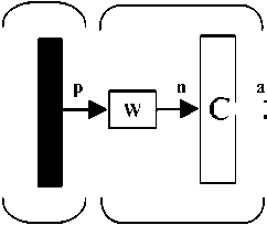
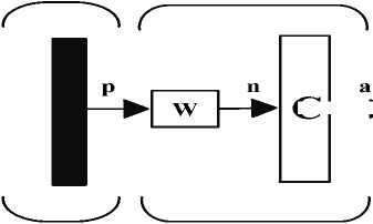
A competitive layer is displayed in Figure 2.

Input     Competitive Layer

C a=Compt(Wp)

Figure 2. Competitive layer.

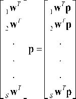
As with the Hamming network, the prototype vector is stored in the rows of W. The net input n calculates the distance between the input vector p and each prototype iw. The net input ni of each neuron I is proportional to the angle 0 i between P and the prototype vector iw :

L cos 0

L cos 0

L cos 0

The competitive transfer function assigns one output with value 1 to the neuron whose weight vector points in the direction closest to the input vector. In biological neural networks, neurons are typically arranged in twodimensional layers, in which they are densely interconnected through lateral feedback. In biology, a neuron reinforces not only itself, but also those neurons close to it. Typically, the transition from reinforcement to inhibition occurs smoothly as the distance between neurons increases. Biological competitive systems, in addition to having a gradual transition between excitatory and inhibitory regions of the on-center/off-surround connection pattern, also have a weaker form of competition of a single active neuron (winner), biological networks generally have “bubbles” of activity that are centered around the most active neuron. In order to emulate the activity bubbles of biological systems, without having to implement the nonlinear on-center/off-surround feedback connections, Kohonen designed the following simplification. His self-organizing feature map (SOFM) network first determines the winning neuron i* using the same procedure as the competitive layer. Next, the weight vectors for all neurons within a certain neighbourhood of the winning neuron are updated using the Kohonen rule,

.w ( q ) = , w ( q - 1) + « ( p ( q ) - , w ( q ^{- 1))} i ^e N * (d ) (4)

When a vector p is presented, the weights of the winning neuron and its neighbours will move toward p. The result is that, after many presentations, neighbouring neurons will have learned vectors similar to each other.

• B.    Proposed Modified SOFM

In the proposed architecture the neurons have arranged in a two-dimensional pattern (pixels in the image). Each time a vector (columns of the input image) is presented, the neuron with the closest weight vector will win the competition. The winning neurons and its neighbours (Next column of weight vector) move their weight vectors closer to the input vector. For this work we are using a neighbourhood with the next column of the weight vector. Competitive layer used in the proposed method is shown in Figure 3.

Input

Competitive Layer

C ni = -||iW-p|| a=Compt(Wp)

Figure 3. Competitive layer used in the proposed method.

As with the competitive network, each column of neuron in the this layer of the proposed network learns a prototype vector, which allows it to classify a region of the input space. However, instead of computing the proximity of the input and weight vectors by using the inner product, we using of the distance directly. One advantage of calculating the distance directly is that vectors need not be normalized. The net input of the proposed network will be

n,=- Lw - PII

Or, in vector form,

¹¹ 1^{w -} P ¹¹

II 2W — P IIII S1 w-P II

The output of the proposed network is a = Compt(n)

Therefore the number of columns of the neurons whose weight vector is closest to the input vector (that is column of the input image) will output a is 1, and the other number of columns of the neurons will be 0. Any time we compute the distance directly of one column of the input image with total of columns of weight matrix. Smallest distance directly is winner in competition. Winner column of the weight vector w (q) and next column w (q+1) are updated so the probability of winning next column is increased. In the proposed method possible winning is for winner column and the next column thus allow next column neurons be win the competition so after a few iterations continuously some of the columns of the weight matrix are winner in competition at the end of the iteration input image is estimated and compressed in the number of lower columns than the input image. So input image is compressed in the weight matrix in continuous columns that are lower than the number of columns of the original image. Now in following the proposed network learning is presented. The Kohonen rule is used to improve the network. First, if p is classified correctly, then we move the column weight of the winning neurons and next column weight toward p.

^{w (} q ) = w ⁽ q ^- 1) + « ⁽ p ^- w ⁽ q ^- 1)) (8) w ( q + 1) = w ( q ) + a ( p - w ( q ))

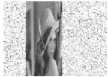
As seen in the Figure 4 input image is estimated by the proposed Modified SOFM in compressed state. The number of winner columns in weight matrix is about 43 to 111, but input image has 200 columns based on the proposed method estimated input image is created in the weight matrix (neurons) by these winner columns i.e. by 68 columns.

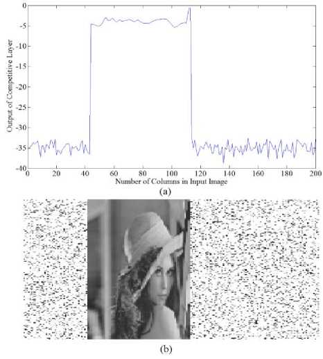
Figure 4. (a) Output of the competitive layer, (b) estimated input image on neurons.

Figure 5 shown a number of the winner columns in final iteration the number of winner columns in weight matrix is about 43 to 111. As seen in the figure order of winner columns are incrementally this is based on the proposed learning rule as explained in this section, in competitive layer competition is between columns of neurons. So closest columns of neurons (weight matrix) to column of the input image that is as input vector is winner thus winner column and next column of weight matrix are updated.

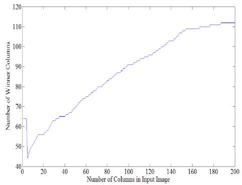
Figure 5. Number of the winner columns in final iteration.

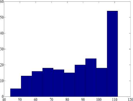
As seen in Figure 5 by using the proposed learning rule winning probability of the next column is increased and winner columns are neighbourhood (incrementally) in the end iteration input image is formed by winner columns that a number of these columns are lower than the number of input images. Fig.6 shown histogram of the number of the winner columns in the proposed MSOM in this example number of the winner columns is between 43 to 111.

Number of Winner Columns

Figure 6. (a) Histogram of the number of the winner columns.

As seen in the figure approximately probability of winning of any interval of columns are equal.

• C.    Second stage of the proposed method based on Back-propagation

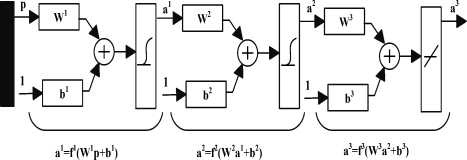
  The demonstration of the limitations of single-layer neural networks were a significant factor in the decline of interest in neural networks in the 1970s The discovery and widespread dissemination of an effective general method of training a multilayer neural network. In this part of the paper, we shall discuss this training method, known as back-propagation (of errors) or the generalized delta rule. It is simply a gradient descent method to minimize the total squared error of the output computed from the net. The very general nature of the back-propagation training method means that a back-propagation net can be used to solve problems in many areas. The training of a network by back-propagation involves three stages: the feed forward of the input training pattern, the back-propagation of the associated error, and the adjustment of the weights. After training, application of the net involves only the computations of the feed forward phase. Even if training is slow, a trained net can produce its output very rapidly. Numerous variations of back-propagation have been developed to improve the speed of the training process. More than one hidden layer may be beneficial for some applications, but one hidden layer is sufficient [11]. Figure 7 shows back-propagation network.

In forward propagation

Input Image      First layer

Hidden layer

Output layer

That p is input vector

Figure 7. Back-propagation network.

a ⁰ = p

a m + i = f m ^{+ 1}( w m + 1 a m + b m ^{+ 1})

a = a

M

In backward propagation

for m = 0,1,..., M - 1

The back-propagation is directly applied to image compression. The compression is achieved by estimating the value of X, the neurons in the hidden layer less than that of neurons in both the input and output layers. The “N” is the number of neurons in the input or output layer and the “X” is the number of the hidden layer. The input image is split up into a number of columns, each column has “N” pixels, which is equal to the number of input neurons.

• D.    Algorithm of the back-propagation network

An activation function for a back-propagation net should have several important characteristics: It should be continuous, differentiable, and monotonically nondecreasing. Furthermore, for computational efficiency, it is desirable that its derivative be easy to compute. For the most commonly used activation functions, the value of the derivative (at a particular value of the independent variable) can be expressed in terms of the value of the function. Usually, the function is expected to saturate, i.e., approach finite maximum and minimum values asymptotically. The performance index of this algorithm is

F ( x ) = E[e^Te ] = E[(t - a)^T (t - a )] (9)

Also approximate on the performance index back propagation is

F(x) = eT (k)e(k) = (t(k) - a(k))T (t(k) - a(k))

The sensitivity of F ˆ to change in the ⁱth element of the net input at layer m.

SM = -2FM (nM )(t - a)

S m = F m ( n m )( W ^{m + i} )^Ts^{m + 1}     for m = M - 1,..,2,1

Where fm(nm)       0       ...0

0 fm(nm)  ...0

F ^m ( n ^m ) =

0           0       ... f ^m ( n m ^m )

f ^m (n₃ ) =

d f^m (n* m )

d n_y

m

In final weight update (approximate steepest descent)

w m (k +1) = wm (k) - aSm (am-1)T(13)

b m (k +1) = b m (k) - aSm(14)

In proposing a method implemented algorithm is:

• a ⁰ = p

The output of the first layer is

• a ¹ = f ¹ ( w ¹ a ⁰ + b ¹ ) =

log sig ( Г w ¹ 1      Г a ⁰ 1    +F b ¹ 1     ) = Г a ¹ 1

L J 200*200 L   J 200*1 L   J 200*1⁷ L J 200*1

SF m dnm

d F d n m d F d n”

The output of a hidden layer is

d F d n_S”

a2 = f 2(w2 a1 + b2) = log sig([w2 ] ,200 [a1 ]20OT +[b2 ] .,) = [a2 ] x*200        200*1           x*1             x*1

That x is the number of neurons in the hidden layer. The third output layer is, a 3 = f 3(w 3 a2 + b3) = purelin ([ w3 ]    [ a2 ]  +[b3 ]   ) = [ a3 ]

200* x        x *1          200*1            200*1

The error would then be,

e — t — a2

^{— [ t ]} 200*1

—

^{[ a  ]} 200*1

^{— [} e ] 200*1

The next stage of the algorithm is to back propagation the sensitivities. Before we begin the back propagation, we will need the derivatives of the transfer functions. For the first layer,

f ’( n ) — d (^ dn 1 + e

— n

)

^——(1--)(—)

1 + e ^{— n}        1 + e ^{— n}  1 + e ^— n

(1 — a 1 )( a 1 )

For the hidden layer we have f 2( n ) — (1 — a 2X a2)

For the third layer we have

. f ³( n ) — d ( n ) — 1

dn

We can now perform the back-propagation. The starting point is found in the third layer, using Eq (12):

S ³ — — 2 F ³ ( n ³)( t — a ) — — 2 [ f ³( n ³) ] ( t — a )

S ² — F ²( n ²)( w ³) T S ³ —

"(1—ax 2)(ax 2)          0          ...            0"

0         (1—a22)(a22) ...0

.                     ’                             .                      [ s ³ ]

L J 200*1

.                                    .                     ....

.                                                  ..

-        ^{0                 0}           ...   ^{(1 —} a 2002⁾⁽ a 2002 ) _ 200*200

And for S1,

S ¹ — F 1 ( n ')( w ²) T S ² —

"(1—ax 1)( a 1)         0         ...           0"

0         (1—a2 1)(a2 1)  ...0

■                    ■                             .                       [ S ² ]

.                      .             ...                .                          L J 200*1

...

_       ^{0                0}          ...   ^{(1 —} a 2001⁾⁽ a 2001 ) _ ₂₀₀*₂₀₀

The final stage of the algorithm is to update the weights. For simplicity, we will use a learning rate α=0. 66. From (13) and (14) we have:

w3 (1) — w3 (0) — aS3 (a 2) T w2 (1) — w 2 (0) — aS 2 (a1) T w 1(1) — w 1(0) — aS 1( a 0) T

And for bias b3 (1) — b3 (0) — aS3

b ² (1) — b ² (0) — aS ²

b 1 (1) — b 1 (0) — aS ¹

We continue to iterate until the difference between the network response and the target function reaches some acceptable level. After training of this network reconstructed image is achieved.

IV . COMPARISON AND EXPERIMENTAL RESULTS

The quality of an image is measured using the parameters like Mean Square Error (MSE) and Peak Signal to Noise Ratio (PSNR). The MSE and the PSNR are the two error metrics used to compare image compression quality. These two parameters define the quality of an image reconstructed at the output layer of the neural network. The MSE between the reconstructed image and original image should be as small as possible so that the quality of reconstructed image should be near to the original image. The MSE metric is most widely used for in simple to calculate, MSE is computed by averaging the squared intensity difference of reconstructed image RI and the original image, OI.

MN

MSE — ^7 EZL Oi (i, j)—Ri (i, j) J

That N, M are the dimensions of the image.

Then based on MSE the PSNR is calculated, so the PSNR is defined as follows:

PSNR —10 log,0 L2552 / MSEJ (db)

PSNR represents a measure of the peak signal to noise ratio the higher the PSNR, the better the quality of the compressed or reconstructed image. The computer system used for the investigation had the specifications of 2.20GHz CPU, 2.00GB RAM and the MATLAB version 7.4 was applied for the study. The proposed algorithm is simple and high speed. The performance of the network has been evaluated using some standard images. Total images in this work are 200*200 pixel In the follow achieved result of different image are demonstrated. Figure 8 shows the Lena Image original image and two reconstructed images with α=0.66 and α=0.1 that α is learning rate in back-propagation algorithm. Table I shows achieved result of Lena image.

Original image

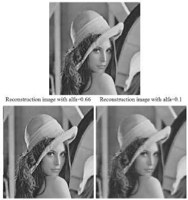
Figure 8. Lena Image and two reconstructed images with α=0. 66 and α=0.1 by the proposed method.

TABLE I: RESULTS OF LENA IMAGE.

Image 200*200	PSNR (db)	MSE	Time (Sec)	Bits    per pixel
Lena	67.7513	26.6388	18.2768	2

Figure 9 shows the Barbara Image original image and two reconstructed images with α=0.66 and α=0.1 that α is learning rate in back-propagation algorithm.

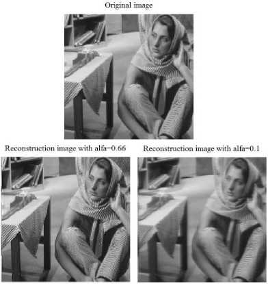
Figure 9. Barbara Image and two reconstructed images with α=0. 66 and α=0.1 by the proposed method.

Table II shows achieved result of Barbara image.

TABLE II: RESULTS OF BARBARA IMAGE.

Image 200*200	PSNR(db)	MSE	Time (Sec)	Bits   per pixel
Barbara	68.1886	25.3309	15.9491	2

Figure 10 shows Peppers image original image and two reconstructed images with α=0.66 and α=0.1 that α is learning rate in back-propagation algorithm. Table III shows achieved result of the peppers image.

TABLE III: RESULTS OF PEPPERS IMAGE.

Image 200*200	PSNR (db)	MSE	Time (Sec)	Bits per pixel
Peppers	69.2541	22.4065	18.3992	2

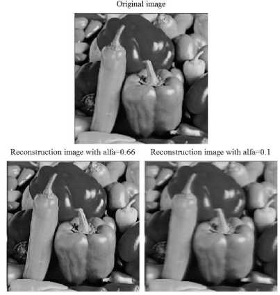
Figure 10. Peppers image and two reconstructed images with α=0. 66 and α=0.1 by the proposed method.

Figure 11 shows the Baboon image original image and two reconstructed images with α=0.66 and α=0.1 that α is learning rate in back-propagation algorithm. Table IV shows achieved result of the Baboon image.

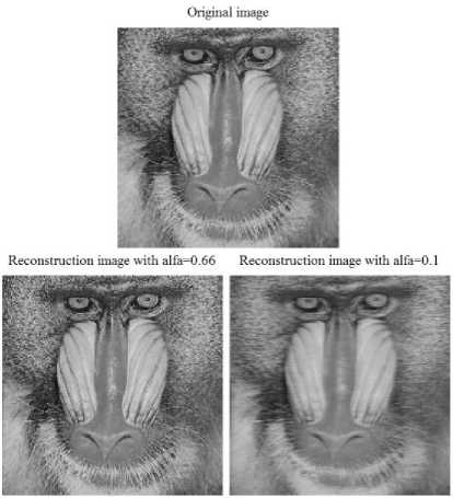
Figure 11. Baboon image and two reconstructed images with α=0. 66 and α=0.1 by the proposed method.

TABLE IV: RESULTS OF BABOON IMAGE.

Image 200*200	PSNR(db)	MSE	Time (Sec)	Bits  per pixel
Baboon	67.3420	27.9241	15.4096	2

Table V shows the results of different methods.

TABLE V: RESULTS OF DIFFERENT METHODS.

45 О 1	ей	0J N (Я	Pi сц	S н	ш с/> 3
[8]	Lena	256*256	28.91	182	---
[8]	Pepper	256*256	29.04	188	---
[12]	Lena	256*256	26.33	---	---
[5]	Lena	256*256	24.7	---	---
[9]	Lena	256*256	45.13	---	---
[10]	Lena	256*256	38.6035	3270.101	20.127
[10]	Pepper	256*256	32.2945	3983.112	24.29

As seen in the above tables the proposed method has High-speed over other existing works in the image compression.

• V. CONCLUSION

In this paper we construct a high-speed image compression based on the combination of modified selforganizing map and back-propagation neural networks. The proposed method is based on two major parts, the first partition is the MSOFM and the second partition is back-propagation algorithm. In the first stage by MSOFM and the proposed weight update method estimated a distribute function of the input image in lower dimensions by neurons (weight matrix) this is first information compression and back-propagation is second stage of the image compression. The results show design works properly and compare to previous implementation it is able to work at higher speeds. Speed and PSNR are two features of the proposed method over other existing works.