Histogram Bins Matching Approach for CBIR Based on Linear grouping for Dimensionality Reduction

Автор: H. B. Kekre, Kavita Sonawane

Журнал: International Journal of Image, Graphics and Signal Processing(IJIGSP) @ijigsp

Статья в выпуске: 1 vol.6, 2013 года.

Бесплатный доступ

This paper describes the histogram bins matching approach for CBIR. Histogram bins are reduced from 256 to 32 and 16 by linear grouping and effect of this dimensionality reduction is analyzed, compared, and evaluated. Work presented in this paper contributes in all three main phases of CBIR that are feature extraction, similarity matching and performance evaluation. Feature extraction explores the idea of histogram bins matching for three colors R, G and B. Histogram bin contents are used to represent the feature vector in three forms. First form of feature is count of pixels, and then other forms are obtained by computing the total and mean of intensities for the pixels falling in each of the histogram bins. Initially the size of the feature vector is 256 components as histogram with the all 256 bins. Further the size of the feature vector is reduced to 32 bins and then 16 bins by simple linear grouping of the bins. Feature extraction processes for each size and type of the feature vector is executed over the database of 2000 BMP images having 20 different classes. It prepares the feature vector databases as preprocessing part of this work. Similarity matching between query and database image feature vectors is carried out by means of first five orders of Minkowski distance and also with the cosine correlation distance. Same set of 200 query images are executed for all types of feature vector and for all similarity measures. Performance of all aspects addressed in this paper are evaluated using three parameters PRCP (Precision Recall Cross over Point), LS (longest string), LSRR (Length of String to Retrieve all Relevant images).

Еще

Histogram bins, linear grouping, count of pixels, total intensities Mean, PRCP, LS, LSRR

Короткий адрес: https://sciup.org/15013201

IDR: 15013201

Текст научной статьи Histogram Bins Matching Approach for CBIR Based on Linear grouping for Dimensionality Reduction

Published Online November 2013 in MECS

Image retrieval is one of the vast areas of research where researchers are working for various different aspects of content based image retrieval (CBIR). Major components to be addressed in CBIR are feature extraction, feature matching, query specification and performance evaluation. Feature extraction mainly based on the three primary contents of the image that are color, texture, and shape [1]-[4].There are three major categories of texture -based techniques, namely, probabilistic/statistical, spectral, and structural approaches. Shape representations can be categorized into two types as boundary based or region based. A boundary based representation uses only the outer boundary characteristics of the object, while a region -based representation uses the entire region. Shape features may also be local or global. Local shape features are obtained from the subpart of the image or object whereas global shape feature considers the entire object. [5]-[7]. Color is most widely used visual feature which is simple and robust to represent. Various techniques are developed in different color spaces. Focusing on these primary contents individually and by combining them various methods are designed and developed for feature extraction in image retrieval and pattern matching applications. [8]-[10]. Instead of using only one content for feature representation, it has been found by many researchers that combination of them like, color with texture or color and shape vice versa or combining all three produces better results [7-8], [11][13]. Many have worked with partitioning of an image into different regions then for each region the color histogram will be computed called local histograms. These histograms then will be used as feature vectors for comparing the images. Various techniques have been invented for image retrieval based on histogram processing. Histogram is one of the simple features of the image that takes simple computations and reduces the computational complexity. It is widely used in CBIR field because of the property that it is invariant to scaling and rotation [14]-[16]. In this paper the proposed methods are mainly focusing on the color histogram technique. Work done in this paper is experimented with database of 2000 RGB images. It includes 20 classes where few classes are taken from Wang database [17]. Each database image will be separated into R, G and b components and for each component a histogram will be computed separately. Further these R, G and B histogram bins used as feature vectors and also by computing different features from histogram bins data new features are obtained and feature vector databases are prepared for all 2000 images in the database. Work proposed in this paper is organized as follows. Section II describes algorithmic view of the proposed techniques for feature extraction phase along with preprocessing work done. Section III discusses the similarity measures used for image indexing and retrieval along with the performance evaluation parameters. Section IV presents the experimental set up and Section V presents the results and discussions followed by conclusion in Section VI.

II. Algorithmic view of the Proposed Techniques

Proposed algorithms are designed for feature extraction basically focusing on the color contents of the image. Color content is the primary image visual feature which is simple and robust to extract. It is invariant to scaling and rotation transformation. Color feature can be represented in various different color descriptor formats such as color coherence vector, color structure, color spaces, cumulative histograms, local color histograms Global color histograms, Color correlogram etc [15][18].

A. Histogram Histogram

Image histogram is a graphical representation of the intensity distribution in a digital image. In simple words image histogram is just a bar graph of pixel intensities. Pixel intensities are plotted along with the x-axis and numbers of occurrences for each of these intensities are plotted across y axis .

The purpose of a histogram is to take the data (pixels-grey level information) that is collected from a image and then display it graphically to view the distribution of the data. Histogram gives summary of count of pixels in the number of bins. Histogram bins are representing the no of grey levels in the image. By default Matlab generates 256 bins for the image histogram that represents 0 to 255 intensity levels of the image. [19-20].

We are using the color histograms for the image representation and comparison. We follow the following framework based on color histograms for the image under feature extraction process. Different aspects considered for this histogram based features and their use are explained below.

B. Feature Extraction Frame Work for Proposed

Algorithms

Framework shown in Figure. 1 is briefing the idea of proposed algorithms as part of feature extraction phase executed and explored in this paper. There are different types of feature vectors computed and each type of feature vector is stored in separate databases. To have the multiple types of features, the algorithms used for feature extraction and representation are explained below. First two, are the basics or say common steps for all types of features to be extracted. Step three onwards there are little variations used in histogram bins data extracting and representing process. One variation is based on the dimension of the feature vector. Other one is the form of using the histogram bins data.

As shown in Figure 1 Feature extraction starts with first two steps:

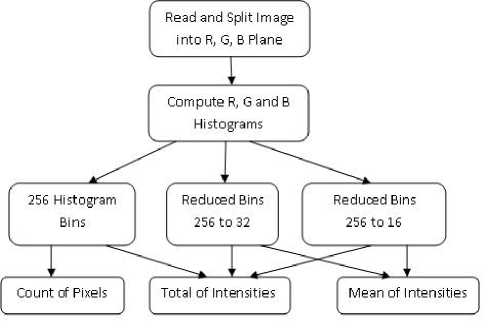
Figure 1. Histogram Based Feature Extraction Framework

Step 1: Read the image from database and split it into R, G and B planes.

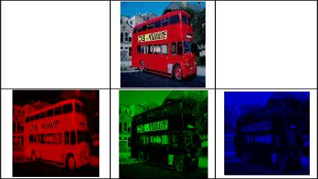
Figure 2. Bus Image with R, G and B planes Separated

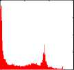
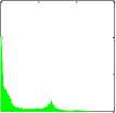
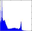
Step 2: Compute the R, G and B histograms

Original Red Image Histogram

0 100 200 300

Original Green Plane Histogram 1500

Original Blue Plane Histogram

0 100 200 300

Figure 3. R, G and B Plane Histograms for Bus Image

Step3: Each histogram (In MATLAB) is represented by 256 bins for each intensity from the range 0 to 255. Initially we have used all 256 bins data as feature vector. Image features details are given as follows.

Step 3 A: Feature Dimension: 256 Bins

Feature vector type

i. Count of Pixels,
ii. Total of Intensities into each bin:

R_total256, G_total 256, B_total256.

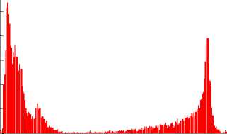
Step 3 B: Reducing the size of feature vector from 256 to 32 and 16 by simple linear grouping of 8 and 16 histogram bins respectively. It is shown in Fig.4.

0 50 100 150 200 250

No of Bins

Figure 4. Original Histogram 256 Bins

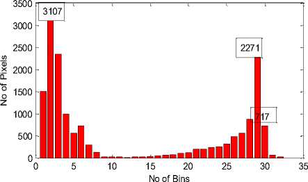
Figure 5. Linear Grouping of 8 bins of Histogram for Dimension Reduction from 256 to 32 Bins

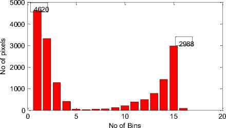
Figure 6. Linear Grouping of 16 bins of Histogram for Dimension Reduction from 256 to 16 Bins

According to this we are linearly grouping the 8 consecutive bins of histogram till 256. Linear grouping is nothing but adding total pixels falling in those consecutive 8 bins. This gives the set of 32 bins that is what the dimension of feature vector reduced to 32 bins. Tonal contents in the collected as count of pixels are represented in following forms to be used as feature vectors.

Step 3 C Feature Dimension: 32 Bins Feature vector type

i. Count of Pixels,
ii. Total of Intensities into each bin:

R_total32, G_total32, B_total32.

iii. Mean of In tensities:

R _ Mean32 , G_Mean32, B_Mean32.

Step 3 D Feature Dimension: 16 Bins

Feature vector type

i. Count of Pixels,
ii. Total of Intensities into each bin:

R_total16, G_total16, B_total16.

iii. Mean of In tensities:

R _ Mean16 , G_Mean16, B_Mean16.

Based on these steps different types of feature vectors are extracted with respect to color and the way of processing and representing the bins data. After feature extraction the next important phase we come across is feature matching between database and the query image. This comparison process is carried by means of similarity measures which are discussed as follows.

II I. Similarity Measures and Performance evaluation Parameters

These both the aspects are essential to test the flawless working of the system and to evaluate the performance of the proposed approaches based on these factors on some common ground.

A. Similarity Measures:

Once the preprocessing of feature vector database is done the user can fire the query as an example image to the system. System computes the feature vector for the same. Query image and database image feature vectors are then compared by means of the similarity measures. It is responsible for the finding the distance between them which will be interpreted in terms of relevancy with each other [21]-[25]. In this paper we have worked out five distance measures and one similarity measure i.e angular distance. The first five includes Minkowski distance from order 1 to order 5(Nomenclature used for them are L1 to L5) and Cosine correlation distance is used as sixth distance measure.

Minkowski Distance :

( ^ ⁷

Dist DQ = ^ D i - Qi\

V I = 1 7

Where ‘r’ is a parameter, ‘n’ is dimension and ‘I’ is the component of Database and Query image feature vectors D and Q respectively.

To try effect multiple similarity measures Minkowiski order parameter r is used from order 1 to 5.

(1)

Cosine Correlation Distance :

(D (n )MQ ( n ))

where D(n) and Q(n) are Database and Query feature Vectors resp.

It is computed in terms of cos θ as angular distance measure between query and database feature vectors.

Equations of the similarity measures used in this paper are given above in equation 1 and 2.

B. Performance Evaluation Parameters

Once the system is ready to face the query from the user it will compute feature vector for it. This feature vector will be compared with all database images (features) by means of similarity measure. This process generates set of images as an output for the query fired to the system. It contains the images relevant to query or some images which are irrelevant. Ideally the system should not contain any irrelevant image. But still this area has scope for researchers to work for achieving 100 % results where retrieval set for any given query will have only relevant images. Whenever any new approach is being explored it should be evaluated with some scale or parameter so that the efficiency of the approach can be determined [26]-[27]. It will also help the users and the researchers to interpret that how far they from the ideal CBIR system. To do the same, we have used three parameters to evaluate the performance of the system through all possible perspectives of CBIR users. Three parameters used are namely PRCP (Precision Recall Cross over Point), LS (Longest String), and (LSRR) i.e Length of String to Retrieve all Relevant Images). Equations 3, 4 and 5 are defining these three parameters.

PRCP : Precision Recall Cross over Point

Where, precision and recall are defined as follows in equation 3 and 4.

IV. Experimentation Details

Performance of the CBIR systems will be evaluated when the query enters into the system and system generates the retrieval result for it. Speed of retrieval depends on the technique used for feature extraction and also the preprocessing done. Preprocessing done for any system is either preparing the feature vector database for all database images or the processing the query image based on some common criterion to bring it in acceptable format for the system.

A. Preprocessing Work:

As preprocessing work of this paper, we have executed the proposed algorithms for all the database images (i.e 2000 images) Based on the algorithms multiple feature vector databases (RGB, total of intensities, mean of intensities, count of pixels etc) for three different sizes of features i.e 256, 32 and 16 executed are prepared. Image database details are given as follows:

B. Image Database

To execute and check the performance of proposed algorithms experimentation is carried out over database of 2000 BMP images. It includes images from 20 different categories, where few categories are added from Wang database. Sample image from each of the 20 classes of images is shown below in Figure 5.

Relevant Retreived Ιmages

Precision =----------------------------

All Retrieved Images

Recall =

Relevant Retreived Images

All Relevant In Database

Length of string to retreive all relevant Total images in database

C. Query Specification

As the feature vector databases are ready for all images in the database, to complete the experimentation process, A query should be fired to the system to retrieve the relevant images. This phase is called query specification. There are many ways to fire the query to the system. It includes query by content, query by class (category), query by example image etc [28]-[29]. In this experimentation the query specification used is “query by example image” approach. To check the working and active role of the system all approaches

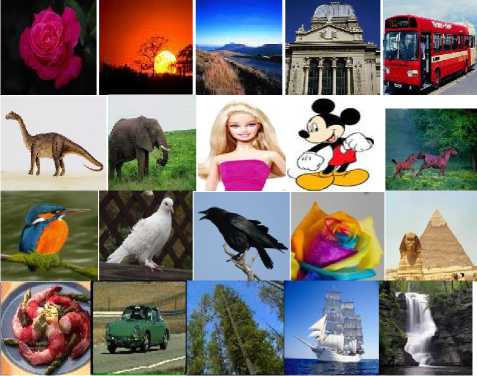
Figure 7. Sample Images from database of 2000 BMP images from 20 classes designed are executed with 200 query images. Set of 200 query images includes the 10 images selected randomly from each of the 20 classes of database. All approaches are executed with each of the six similarity measures (i.e first five orders of Minkowski distance (L1 to L5) and cosine correlation distance (L6) namely L1 to L6 and tested with same set of 200 images and so that their performances can be evaluated and checked on common ground.

V. Results and Discussion

This section is presenting the results obtained for execution of each query for each approach with each similarity measure named as L1 to L6 (based n size, type of feature). The results discussed, observed, and evaluated using PRCP, LSRR, and LS parameters.

A. PRCP: Precision and Recall Cross Over Point

As said earlier this parameter is cross over point of conventional parameters precision and recall. In many CBIR systems it has been observed that when precision is high recalls falls down and if recall is high then precision falls down. This is because it depends on the threshold selected for the distances sorted in ascending order to retrieve the set of images for the given query.

In this paper instead of taking or determining the threshold on trial and error basis we used the following logic to retrieve the images. What we do here is we sort the distances of query image with database images in ascending order. In this experimental set up, total length of sorted distances is 2000. Then we select first 100 images out of these 2000 images and we take the count of query relevant images from this 100 only. As we have 100 images of each class in the database and the count of images relevant to query is also taken out of 100; it generates the cross over point where precision and recall both are same.

PRCP =1 is indication of the ideal system performance where we can say that set of images retrieved from the database contains all the images in the database which are relevant to query. (This set do not contains a single irrelevant image).

PRCP = 0 is the indication of worst case performance of the system where the retrieved set of images does not contain a single image which is relevant to query. It has all the images which are irrelevant to query.

Following tables I to VI are showing the results obtained for parameter PRCP for 256 bins of histogram for feature vector type count of pixels and table VII to XII are for total of intensities. Each table is giving the results obtained for each of the six similarity measures from L1 to L5 and CD. Summary on observing these results given tables from I to XII is highlighted in Table XIII. Same process is repeated for 32 and 16 bins and the results for them are shown in table XIV to XVII. In all the tables each value in first three columns is out of 1000( i.e total execution of 10 queries from each class).

TABLE I. PRCP: Total GL 256 Bins L1

Query Class	R	G	B	R OR G OR B
Flower	242	431	242	639
Sunset	294	112	406	579
Mountain	92	86	132	234
Building	155	179	159	329
Bus	164	185	224	412
Diansour	513	563	454	638
Elephant	265	198	234	440
Barbie	566	566	554	684
Mickey	359	408	309	529
Horses	227	191	281	395
Kingfisher	79	68	60	152
Dove	443	441	375	488
Crow	32	47	59	107
Rainbowrose	142	146	116	281
Pyramids	150	115	81	290
Plates	184	190	217	350
Car	194	182	216	409
Trees	277	279	299	416
Ship	203	125	159	316
Waterfall	183	209	238	312
Total	4764	4721	4815	8000

TABLE II. Total GL 256 Bins L2

Query Class	R	G	B	R OR G OR B
Flower	191	389	208	565
Sunset	331	117	326	558
Mountain	87	95	144	238
Building	155	171	146	321
Bus	140	164	205	390
Diansour	479	540	424	593
Elephant	259	217	263	465
Barbie	545	542	543	585
Mickey	295	365	279	438
Horses	230	200	252	376
Kingfisher	77	63	53	142
Dove	283	285	250	326
Crow	54	104	84	198
Rainbowrose	96	119	114	225
Pyramids	159	117	106	306
Plates	216	189	237	390
Car	173	164	215	376
Trees	274	275	281	411
Ship	191	123	170	321
Waterfall	197	202	206	337
Total	4432	4441	4506	7561

TABLE III. PRCP: Total _GL _256 Bins_ L3

Query Class	R	G	B	R OR G OR B
Flower	157	366	203	524
Sunset	317	111	250	512
Mountain	81	101	157	248
Building	159	149	134	311
Bus	109	121	152	297
Dinosaur	510	572	444	618
Elephant	248	216	263	455
Barbie	544	545	543	586
Mickey	302	369	283	435
Horses	228	209	237	367
Kingfisher	81	74	53	148
Dove	158	161	165	212
Crow	72	126	105	245
Rainbowrose	88	104	98	199
Pyramids	184	133	102	338
Plates	193	213	229	409
Car	143	143	204	342
Trees	257	242	269	411
Ship	173	122	179	323
Waterfall	196	175	189	338
Total	4200	4252	4259	7318

TABLE V. PRCP: Total _GL _256 Bins_ L5

Query Class	R	G	B	R OR G OR B
Flower	146	365	209	523
Sunset	313	108	228	491
Mountain	80	101	166	259
Building	157	143	135	310
Bus	101	113	144	286
Dinosaur	513	576	452	628
Elephant	238	208	262	449
Barbie	544	546	544	586
Mickey	302	370	290	439
Horses	227	208	234	366
Kingfisher	78	75	54	149
Dove	146	143	152	205
Crow	77	128	105	250
Rainbowrose	86	99	90	196
Pyramids	187	142	104	346
Plates	188	211	231	415
Car	140	146	198	338
Trees	251	233	261	409
Ship	161	122	176	312
Waterfall	204	170	195	346
Total	4139	4207	4230	7303

TABLE IV. PRCP: Total GL 256 Bins L4

Query Class	R	G	B	R OR G OR B
Flower	182	374	200	544
Sunset	325	117	296	541
Mountain	81	100	154	243
Building	158	164	139	319
Bus	117	132	168	321
Dinosaur	502	559	432	605
Elephant	259	215	261	466
Barbie	541	544	542	585
Mickey	297	366	282	432
Horses	225	205	237	365
Kingfisher	80	69	55	148
Dove	200	201	189	248
Crow	65	122	97	229
Rainbowros	88	110	103	209
Pyramids	176	130	108	327
Plates	198	208	234	400
Car	152	149	209	350
Trees	265	257	277	410
Ship	179	127	175	325
Waterfall	198	190	181	336
Total	4288	4339	4339	7403

TABLE VI. PRCP: Total GL 256 Bins CD

Query Class	R	G	B	R OR G OR B
Flower	178	296	224	517
Sunset	346	113	257	522
Mountain	108	100	136	257
Building	148	140	140	300
Bus	100	100	174	308
Dinosaur	586	685	521	735
Elephant	259	201	233	438
Barbie	577	655	622	750
Mickey	310	427	330	519
Horses	257	232	294	420
Kingfisher	77	65	63	156
Dove	93	133	146	178
Crow	56	95	87	198
Rainbowrose	89	122	92	219
Pyramids	137	111	113	298
Plates	214	195	216	389
Car	191	167	217	394
Trees	228	236	230	361
Ship	160	117	160	289
Waterfall	201	217	215	360
Total	4315	4407	4470	7608

TABLE VII. PRCP: Count of Pixels _256 Bins_ L1

Query Class	R	G	B	R OR G OR B
Flower	369	468	366	645
Sunset	240	82	296	477
Mountain	88	99	142	253
Building	162	187	154	310
Bus	225	380	293	568
Diansour	813	821	686	919
Elephant	309	263	254	480
Barbie	703	637	699	806
Mickey	434	475	393	589
Horses	228	186	255	373
Kingfisher	94	91	62	183
Dove	401	403	399	422
Crow	70	130	124	263
Rainbowrose	143	129	117	270
Pyramids	268	180	116	431
Plates	207	240	245	407
Car	201	193	261	430
Trees	266	311	319	460
Ship	211	146	194	358
Waterfall	217	222	224	326
Total	5649	5643	5599	8970

TABLE IX. PRCP: Count of Pixels _256 Bins_ L3

Query Class	R	G	B	R OR G OR B
Flower	341	442	440	603
Sunset	315	95	260	529
Mountain	95	103	150	270
Building	141	157	124	271
Bus	226	355	244	570
Dinosaur	503	559	432	604
Elephant	321	260	302	518
Barbie	552	545	545	589
Mickey	297	359	277	436
Horses	200	198	210	350
Kingfisher	80	72	62	153
Dove	388	388	375	399
Crow	70	123	98	233
Rainbowrose	86	91	100	189
Pyramids	196	143	119	347
Plates	223	239	231	421
Car	222	189	284	452
Trees	243	289	249	455
Ship	395	117	174	488
Waterfall	260	198	205	394
Total	5154	4922	4881	8271

TABLE VIII. PRCP: Count of Pixels 256 Bins L2

Query Class	R	G	B	R OR G OR B
Flower	351	460	444	609
Sunset	294	83	256	493
Mountain	95	103	141	262
Building	161	168	136	285
Bus	212	381	268	584
Dinosaur	485	553	434	606
Elephant	323	259	292	506
Barbie	557	554	554	596
Mickey	300	365	277	436
Horses	213	188	225	353
Kingfisher	83	75	59	160
Dove	385	388	374	400
Crow	57	111	92	212
Rainbowrose	105	104	113	213
Pyramids	199	140	117	355
Plates	226	237	239	426
Car	192	182	255	420
Trees	264	304	279	471
Ship	321	128	185	423
Waterfall	251	227	220	378
Total	5074	5010	4960	8188

TABLE X. PRCP: Count of Pixels 256 Bins L4

Query Class	R	G	B	R OR G OR B
Flower	343	433	438	600
Sunset	309	98	256	528
Mountain	94	107	148	272
Building	133	149	123	264
Bus	236	343	216	560
Dinosaur	511	571	445	617
Elephant	328	261	302	530
Barbie	553	546	546	590
Mickey	298	358	280	433
Horses	195	202	205	355
Kingfisher	75	71	64	151
Dove	392	388	375	402
Crow	77	125	107	247
Rainbowrose	83	89	102	185
Pyramids	189	147	117	347
Plates	212	239	234	427
Car	254	201	298	482
Trees	237	274	241	447
Ship	419	118	187	524
Waterfall	262	180	197	393
Total	5200	4900	4881	8354

TABLE XI. PRCP: Count of Pixels _256 Bins_ L5

Query Class	R	G	B	R OR G OR B
Flower	345	428	427	593
Sunset	313	100	251	534
Mountain	88	110	151	279
Building	126	145	125	265
Bus	242	339	193	552
Dinosaur	514	578	451	630
Elephant	328	257	303	537
Barbie	553	546	545	592
Mickey	301	363	284	437
Horses	196	207	195	358
Kingfisher	70	73	68	151
Dove	393	390	375	403
Crow	78	128	105	249
Rainbowrose	79	83	99	175
Pyramids	189	153	109	348
Plates	210	229	231	428
Car	268	197	297	495
Trees	233	266	233	440
Ship	421	122	187	529
Waterfall	268	174	189	401
Total	5215	4888	4818	8396

TABLE XII. PRCP: Count of Pixels 256 Bins CD

Query Class	R	G	B	R OR G OR B
Flower	386	459	471	614
Sunset	288	96	235	481
Mountain	97	98	145	267
Building	146	169	129	279
Bus	220	338	254	545
Dinosaur	709	775	598	819
Elephant	309	256	254	469
Barbie	663	717	739	801
Mickey	358	404	317	532
Horses	232	208	238	379
Kingfisher	89	86	64	174
Dove	376	381	372	396
Crow	66	129	126	267
Rainbowrose	93	96	111	197
Pyramids	228	157	120	399
Plates	221	238	240	425
Car	221	193	282	447
Trees	274	325	281	493
Ship	357	132	190	464
Waterfall	221	210	155	331
Total	5554	5467	5321	8779

TABLE XIII. PRCP : L1 to L5 and CD for 256 Bins Count and Total of Intensities

RGB PRCP OR	PRCP : 256 BINS TOTAL OF INTENSITIES
RGB PRCP OR	L1	L2	L3	L4	L5	CD
COUNT	8970	8188	8271	8354	8396	8779
TOTAL	8000	7561	7403	7318	7303	7608

In above results we can see that the results are obtained separately for R, G and B colors. To improve these results further, instead of taking individual results with respect to R, G and B colors ; we have combined them using OR criterion.

OR Criterion: According to this criterion image being retrieved in any one color will be retrieved in the final set. (i.e. R OR G OR B). It has brought very good improvement in the retrieval set of images similar to query. If we see the total retrieval of 200 query images for each individual color we found that the values are less than 5000. But after applying OR criterion we could retrieve more than 7000 relevant images for the total execution of 200 query images.

We have followed this application of OR criterion for execution of all 200 query images with respect to each of the six similarity measures. This is done for both types of feature vectors i.e count of pixels and total of intensities.

Summary of the results obtained for 256 bins for each similarity measure are given in table XIII. Here we can see that the best results are highlighted in yellow color. We found that here L1 and CD measures proving best among all. The best result obtained is 8970 out of 20000, for count of pixels with L1 measure. It means precision and recall is reached to 0.44.

Next, we have executed the same set of 200 query images for the feature vectors Total of intensities and mean of intensities with dimension 32 and 16 bins for red, green and blue intensities separately. Results obtained for red, green and blue colors considered separately are observed and here also we thought of applying the OR criterion to combine and refine these results so that retrieval can be improved. Following tables XIV to XV are presenting the results for 32 bins and tables XVII and XVIII for 16 bins after applying the OR criterion for all six distance measures.

TABLE XIV. PRCP: TOTAL_32 BINS : R OR G OR B

Query Class	L1	L2	L3	L4	L5	CD
Flower	629	547	522	500	492	499
Sunset	575	553	547	532	525	492
Mountain	235	241	239	239	240	251
Building	332	321	319	300	298	299
Bus	430	410	352	330	314	309
Dinosaur	986	972	974	976	979	964
Elephant	438	466	462	463	462	409
Barbie	692	635	627	629	625	753
Mickey	537	494	489	484	484	527
Horses	390	369	355	350	347	404
Kingfisher	163	151	154	158	158	161
Dove	489	365	309	280	269	205
Crow	174	240	257	271	275	237
Rainbowrose	275	238	221	226	221	218
Pyramids	304	333	347	352	365	296
Plates	346	362	374	379	385	356
Car	409	385	369	371	364	409
Trees	411	402	395	404	404	360
Ship	320	321	320	313	308	288
Waterfall	307	330	334	328	326	351
Total	8442	8135	7966	7885	7841	7788

Table XV. PRCP : MEAN: 32 BINS : R OR G OR B

Query Class	L1	L2	L3	L4	L5	CD
Flower	613	608	604	606	606	610
Sunset	256	250	245	236	237	235
Mountain	304	328	339	338	337	318
Building	386	373	366	362	362	372
Bus	438	429	409	394	385	418
Dinosaur	368	372	369	368	360	371
Elephant	583	558	540	537	528	560
Barbie	520	508	483	439	438	473
Mickey	467	456	457	452	449	405
Horses	430	394	385	374	374	396
Kingfisher	108	126	134	147	149	125
Dove	287	339	357	357	353	346
Crow	258	245	253	253	252	242
Rainbowrose	271	251	227	214	216	253
Pyramids	323	291	280	276	273	280
Plates	498	507	495	476	471	509
Car	353	408	435	445	448	400
Trees	413	370	356	353	349	375
Ship	272	269	265	275	274	274
Waterfall	544	494	456	433	429	495
Total	7692	7576	7455	7335	7290	7457

TABLE XVI PRCP : L1 to L5 and CD for 32 Bins Total and Mean of Intensities

RGB PRCP OR	PRCP : 32 BINS
RGB PRCP OR	L1	L2	L3	L4	L5	CD
TOTAL	8442	8135	7966	7885	7841	7788
MEAN	7692	7576	7455	7335	7290	7457

Table XVII. PRCP: TOTAL_16 BINS R OR G OR for similarity measures L1 TO L5 and CD:

Query Class	L1	L2	L3	L4	L5	CD
Flower	634	545	514	504	495	503
Sunset	576	549	541	534	533	479
Mountain	236	247	242	244	249	243
Building	329	322	311	304	299	290
Bus	442	417	379	359	338	332
Dinosaur	973	951	951	954	957	956
Elephant	433	440	445	440	434	392
Barbie	693	663	651	649	650	694
Mickey	538	503	492	489	490	507
Horses	392	361	348	344	340	394
Kingfisher	179	161	160	160	163	169
Dove	491	390	350	329	318	213
Crow	263	281	290	291	295	278
Rainbowrose	273	252	235	235	236	225
Pyramids	324	346	368	374	377	310
Plates	332	349	356	365	364	341
Car	408	390	378	371	372	406
Trees	397	387	398	398	400	349
Ship	317	318	323	313	307	292
Waterfall	309	323	322	320	320	343
Total	8539	8195	8054	7977	7937	7716

The next parameters used for evaluation of the proposed algorithms are LS i.e Longest String and LSRR. All 200 query images are executed to obtained results for these parameter with each color R, G and B separately.

B. LS: Longest String

As per the definition of LS parameter the results should be as high as possible to prove the best performance of the system. While retrieving the results of LS we have done the additional analysis for checking the performance of each color R, G and B. We have considered only the maximum LS obtained from the results obtained for all 10 queries from each class for R, G and B colors separately. We have marked the color of the maximum LS. Results obtained for LS with 256 bins approach for total of intensities and counts of pixels are shown in Table XX and XXI respectively. Each value in the tables is out of 100 as we have 100 images of each class in the database.

TABLE XVIII. PRCP: MEAN: 16 BINS : R OR G OR B for similarity measures L1 TO L5 and CD:

Query Class	L1	L2	L3	L4	L5	CD
Flower	622	592	582	576	572	580
Sunset	291	285	282	280	277	258
Mountain	275	279	283	296	302	263
Building	405	406	393	384	382	381
Bus	545	546	534	530	520	516
Dinosaur	750	729	719	714	705	721
Elephant	576	568	537	517	509	558
Barbie	663	611	588	555	540	570
Mickey	495	482	469	462	458	431
Horses	461	473	476	480	470	439
Kingfisher	144	157	161	166	170	148
Dove	373	384	365	359	361	398
Crow	245	267	271	273	274	269
Rainbowrose	263	242	236	221	216	247
Pyramids	307	284	292	290	291	298
Plates	473	462	449	446	435	452
Car	471	479	494	503	509	473
Trees	494	443	417	400	385	443
Ship	296	301	312	320	320	284
Waterfall	514	487	469	452	446	482
Total	8663	8477	8329	8224	8142	8211

TABLE XIX. PRCP : L1 to L5 and CD for 16 Bins Total and Mean of Intensities

RGB PRCP OR	PRCP : 16 BINS
RGB PRCP OR	L1	L2	L3	L4	L5	CD
TOTAL	8539	8195	8054	7977	7937	7716
MEAN	8663	8477	8329	8224	8142	8211

As discussed above the Table XX shows the result of LS with the performance analysis of colors R, G and B. It can be observed in the table that Red color is performing better among three. The maximum LS in all distance measures is from class Dinosaur only (highlighted in yellow color). Observing the results with respect to similarity measures we found that L1 and CD are better as compared to other measures. (AVG is 14.4 for L1 and 11.6 for CD and then next in queue is L2 i.e 11.3).

C. LSRR (Length of String to Retrieve all Relevant)

Same process is applied for the other evaluation parameter i.e LSRR. Here also we have checked the performance of R, G and B colors. Here only minimum of 10 queries from each class is taken into consideration. The only difference between two parameters is that for LSRR the result should be as low as possible; as it is the measure of the length to be traversed to collect all relevant images from database. Table XXII and XXIII are showing the LSRR results obtained for total of intensities and count of pixels for feature vector size 256 bins.

Table XX : Longest String for 256 Bins Total of Intensities

Query Class	L1			L2		L3		L4		L5		CD
Flower	15		G	10	B	18	G	12	G	12	G	13	B
Sunset	16		B	10	B	10	B	9	B	9	B	9	R
Mountain	3		R	4	R	4	R	5	B	4	R	4	R
Building	6		R	4	R	4	R	4	R	4	R	4	G
Bus	10		B	5	B	5	G	6	G	4	R	4	R
Diansour	64		G	65	G	64	G	66	G	66	G	50	G
Elephant	13		R	10	R	9	R	9	R	8	B	7	B
Barbie	20		R	17	B	17	R	17	R	17	R	32	B
Mickey	39		B	17	G	15	G	16	G	17	G	31	G
Horses	14		B	9	B	11	B	11	B	9	G	12	G
Kingfisher	4		G	4	R	4	R	5	R	5	B	4	R
Dove	33		G	16	B	7	G	8	G	8	R	6	B
Crow	5		G	11	G	7	R	8	G	7	G	11	G
Rainbowrose	6		R	4	R	5	B	5	B	4	R	6	R
Pyramids	5		G	5	R	5	R	8	B	8	B	4	R
Plates	6		G	9	B	8	B	6	R	6	R	7	B
Car	7		G	7	G	4	R	5	R	7	R	5	R
Trees	9		G	9	R	11	R	11	R	10	R	11	R
Ship	6		R	4	R	5	R	4	R	4	G	4	R
Waterfall	7		B	6	R	6	R	7	R	6	R	8	R
AVG		14.4		11.3		10.95		11.1		10.75		11.6
R, G, B COUNT	6 , 9 , 5			9 ,4 , 7		11 , 5, 4		9, 6, 5		10 , 6, 4		10 , 5, 5

TABLE XXI : Longest String for 256 Bins _ Count of Pixels

Query Class	L1		L2		L3		L4		L5		CD
Flower	15	G	25	B	31	G	28	G	28	G	26	B
Sunset	9	B	8	R	7	R	6	R	8	B	7	R
Mountain	5	R	4	R	5	B	4	G	4	G	4	R
Building	5	R	4	R	4	R	5	R	6	B	5	B
Bus	10	R	12	B	10	B	12	G	12	G	13	G
Diansour	83	G	66	G	64	G	66	G	66	G	75	G
Elephant	16	B	11	R	9	R	12	R	9	R	9	R
Barbie	35	R	17	B	17	R	17	R	17	R	42	R
Mickey	40	G	19	R	17	R	15	R	15	R	38	R
Horses	10	G	10	B	7	R	7	R	7	G	12	B
Kingfisher	4	B	4	G	5	G	4	R	4	G	4	R
Dove	36	R	39	G	38	R	38	R	38	R	43	B
Crow	9	G	6	G	5	G	5	G	5	R	5	R
Rainbowrose	5	R	5	B	4	R	4	R	5	G	6	G
Pyramids	6	B	4	R	4	R	5	R	5	R	6	G
Plates	7	R	6	G	4	R	5	R	5	B	7	G
Car	7	R	13	B	12	B	11	R	10	B	9	B
Trees	9	R	10	B	9	G	8	G	7	R	11	B
Ship	6	G	8	R	9	R	9	R	8	R	8	R
Waterfall	6	R	7	G	8	G	6	R	7	G	6	B
AVG	16.15		13.9		13.45		13.35		13.3		16.8
RGBCOUNT	10 , 5, 5		7 , 6, 7		11 , 6, 3		14 , 6, 0		8 , 8 , 4		8 , 5, 7

TABLE XXII : LSRR for 256 Bins Total of Intensities

Query Class	L1		L2			L3		L4		L5		CD
Flower	33	G		47	B	46	B	46	B	44	B	50	B
Sunset	48	B	65		B	67	B	66	R	66	R	49	R
Mountain	79	R	79		R	79	R	78	R	78	B	70	R
Building	70	R	77		R	76	B	78	R	78	R	78	R
Bus	51	R	72		R	74	R	75	R	75	R	56	B
Dinosaur	68	G	91		G	91	G	91	G	90	G	15	G
Elephant	65	R	79		R	81	R	81	R	81	B	64	R
Barbie	85	R	100		R	100	R	100	R	100	R	32	B
Mickey	87	B	94		R	94	R	93	R	94	R	82	G
Horses	54	B	59		B	58	B	57	B	56	B	60	R
Kingfisher	82	B	81		B	83	R	83	R	83	R	78	B
Dove	62	G	87		R	88	R	88	R	89	R	80	G
Crow	95	R	99		R	99	R	99	R	99	R	97	R
Rainbowrose	82	R	90		R	90	R	90	R	90	R	90	G
Pyramids	83	G	84		R	84	R	84	R	84	R	81	R
Plates	63	G	73		B	79	G	80	B	81	G	63	G
Car	71	R	69		R	73	B	74	B	74	R	64	B
Trees	56	G	76		G	80	G	81	R	81	R	67	R
Ship	65	R	81		R	82	B	82	B	82	B	72	R
Waterfall	62	R	69		G	68	G	68	G	68	G	66	G
AVG	68.05		78.6			79.6		79.7		79.65		65.7
R, G, B COUNT	10 , 6, 4		12 , 3, 5			10 , 4, 6		13 , 2, 5		12 , 3, 5		9, 6, 5

TABLE XXIII : LSRR 256 Bins Count of Pixels

Query Class	L1		L2		L3		L4		L5		CD
Flower	46	G	75	G	61	G	58	G	58	G	48	G
Sunset	76	B	81	R	80	B	58	R	60	R	42	R
Mountain	70	B	84	R	85	R	85	R	85	R	74	R
Building	64	R	80	R	80	B	81	B	81	B	72	R
Bus	34	B	42	G	41	G	46	G	48	G	41	G
Diansour	7	G	87	G	87	G	87	G	87	G	9	G
Elephant	58	G	51	B	61	B	63	B	63	B	52	R
Barbie	15	R	98	R	98	R	98	R	98	R	23	B
Mickey	72	R	90	R	90	R	87	R	88	R	78	G
Horses	69	G	58	G	56	G	59	G	61	G	61	G
Kingfisher	84	R	81	G	83	G	83	G	84	G	80	R
Dove	88	G	98	G	98	G	98	G	98	G	93	B
Crow	94	R	99	R	99	R	99	R	99	R	95	R
Rainbowrose	76	G	93	B	93	B	93	B	93	B	88	G
Pyramids	64	G	75	R	78	R	78	R	79	R	68	G
Plates	57	G	53	G	59	G	63	G	66	G	56	G
Car	63	B	62	B	61	B	52	B	36	B	51	B
Trees	44	B	52	B	60	B	62	B	63	B	47	G
Ship	63	R	66	B	68	B	68	B	67	B	64	R
Waterfall	55	G	56	R	57	G	60	G	64	R	52	G
AVG	59.95		74.05		74.75		73.9		73.9		59.7
R, G, B COUNT	6, 9, 5		8 , 7, 5		5, 8 , 7		6, 8 , 6		7, 7 , 6		7, 10, 3

TABLE XXIV : LS 32 Bins Total of Intensities

LS	L1	L2	L3	L4	L5	CD
MAX	95	92	92	93	93	66
AVG	15	13	12	12	12	11

TABLE XXVIII : LS 16 Bins Total of Intensities

LS	L1	L2	L3	L4	L5	CD
MAX	86	78	79	81	81	23
AVG	15	13	12	12	12	10

Table XXV : LS 32 Bins Mean of Intensities

LS	L1	L2	L3	L4	L5	CD
MAX	18	21	21	33	33	20
AVG	8	9	9	10	9	9

TABLE XXIX : LS 16 Bins Mean of Intensities

LS	L1	L2	L3	L4	L5	CD
MAX	23	24	38	38	38	78
AVG	11	11	12	11	12	12

TABLE XXVI LSRR 32 Bins Total of Intensities

TABLE XXX : LSRR 16 Bins Total of Intensities

LSRR	L1	L2	L3	L4	L5	CD
MIN	6	9	9	9	9	9
AVG	60	69	70	69	68	62

LSRR	L1	L2	L3	L4	L5	CD
MIN	7	10	10	10	10	8
AVG	61	68	68	68	68	62

TABLE XXVII LSRR 32 Bins _ Mean of Intensities

TABLE XXXI : LSRR 16 Bins _ Mean of Intensities

LSRR	L1	L2	L3	L4	L5	CD
MIN	30	32	33	33	33	43
AVG	84	84	85	84	84	84

LSRR	32 LSRR : MEAN
LSRR	L1	L2	L3	L4	L5	CD
MAX	31	37	36	37	39	38
AVG	82	82	82	82	82	84

In LSRR results obtained for 256 bins for total and mean of intensities, as we are interested in the discussion of best i.e Minimum LSRR, we have highlighted the minimum values obtained with respect to each measure in yellow color. The best among them is CD measure where we can see that the average of 20 queries and also the individual results the minimum among all is obtained for CD measure. Next best is L1 i.e AD measure. If we check the color performance here we found red is dominating in total of intensities and green in count of pixels in 256 bins approach.

Same process is applied to 32 and 16 bins approach for total and mean of intensities. Here we have considered only the max and average values for LS and minimum and average for LSRR parameters respectively. These results are shown in tables numbered from XXIV to XXXI. Best results are highlighted in yellow. Color analysis is also done for these results and we found in 32 as well as in 16 bins approach for mean of intensities green is better whereas for total of intensities red is better for parameter LSRR. Similarly in LS parameter we found for mean results red is performing better and for total of intensities blue is better.

VI. Conclusion

This paper explores the simple histogram based bins approach for image retrieval. It actually explores the advantage of simple computations (histogram) for feature extraction process. Dimensionality reduction is also worked out by simple linear grouping of 256 bins of histogram to generate 32 and 16 bins out of 256 bins of original histogram. Performance evaluation is done using three parameters PRCP, LS and LSRR and discussed in previous section in detail. Here are the few conclusions drawn for the proposed algorithms.

The first important factor to be discussed is PRCP results. The best value obtained for PRCP is 8970 for 256 bins with count of pixels. We have extracted the best results from each approach discussed above as follows.

Parameter	256 Bins	32 Bins	16 Bins
PRCP	8970	8442	8663
LS	MAX- 83 AVG- 17	MAX- 95 AVG- 15	MAX- 86 AVG- 15
LSRR	MIN- 9 AVG- 59	MIN-6 AVG- 60	MIN-7 AVG- 61

Now the conclusion can be drawn easily from the above table that 256 bins are performing better as compared to 32 and 16 bins approach, for PRCP and for average value of LS and LSRR. But the computations require for 256 are more than that of 32 and 16 bins approaches which increases the time complexity as well.

As this paper has also explored the use of multiple similarity measures i.e first five orders of Minkowski from 1 to 5 named as L1 to L5 and the sixth one is cosine correlation measure. We have compared their performances too. We found that L1 i.e Absolute distance and CD i.e cosine correlation distances are producing good results as compared to other 4 similarity measures. The next one in queue is Euclidean distance which is most commonly used similarity measure in CBIR systems by many researchers.

Список литературы Histogram Bins Matching Approach for CBIR Based on Linear grouping for Dimensionality Reduction

Raimonodo Schettini, G. Ciocca, Silvia Zuffi, “Content-Based Image Retrieval at the End of the Early Years” Institute of Tecnology, Infomatiche Multimediali-In Color Imaging Science: Exploiting Digital , 2001.
Arnold W.M, Marcel Worring, Simone Santini, “Content-Based Image Retrieval at the End of the Early Years”, IEEE Transactions On Pattern Analysis And Machine Intelligence, Vol. 22, No. 12, December 2000.
V. N. REDDY, K. SATYA PRASAD, “Content Based Image Retrieval Using Local Derivative Patterns”, Journal of Theoretical and Applied Information Technology, 30th June 2011. Vol. 28 No.2, Publication of Little Lion Scientific R&D, Islamabad PAKISTA.
SHI Dongcheng, XU Lan, HAN Ungyan, “Image retrieval using both color and texture features”, The Journal of China Universities Of Posts And Telecommunications Volume 14, Supplement, October 2007.
Hui Yu, Mingjing Li, Hong-Jiang Zhang, “Color Texture Moments For Content-Based Image Retrieval”, Image Processing. 2002. Proceedings. 2002 International Conference on (Volume:3 ) 24-28 June 2002, ISSN :1522-4880, DOI: 10.1109/ICIP.2002.1039125.
Bikesh Kr. Singh1, G. R Sinha, Bidyut Mazumdar “Content Based Retrieval of X- ray Images Using Fusion of Spectral Texture and Shape Descriptors”, 2010 International Conference on Advances in Recent Technologies in Communication and Computing, 978-0-7695-4201-0/10 $26.00 © 2010 IEEE.
Nadia Baaziz, Omar Abahmane, Rokia Missaoui “Texture feature extraction in the spatial-frequency domain for content-based image retrieval”, eprint arXiv:1012.5208, arXiv.org - cs - arXiv:1012.5208.
Ramadass Sudhir , Lt. Dr. S. Santhosh Baboo “An Efficient CBIR Technique with YUV Color Space and Texture Features”, Computer Engineering and Intelligent Systems, ISSN 2222-1719 (Paper) ISSN 2222-2863 (Online) www.iiste.org, Vol 2, No.6, 2011.
Neetu Sharma., Paresh Rawat, and jaikaran Singh, “Efficient CBIR Using Color Histogram Processing, Signal & Image Processing”, An International Journal(SIPIJ) Vol.2, No.1, March 2011.
A Vadivel, A K Majumdar, Shamik Sural, “Perceptually Smooth Histogram Generation from the HSV Color Space for Content Based Image Retrieval”, Int. Conf. on Advances in Pattern Recognition (ICAPR2003), Calcutta, India, 248-251, 2003.
Yixin Chen, James Z. Wang, “CLUE: Cluster-Based Retrieval of Images by Unsupervised Learning”, IEEE Transactions on Image Processing, Vol. 14, No. 8, August 2005.
H.Yu, M. Li, H J. Zhang and J. Feng, “Color Texture Moments for Content-Based Image Retrieval”, Proc. Int. Conference on Image Processing, Volume III, 929-931, 2002.
Gwangwon Kang, Junguk Beak, “Features Defined by Median Filtering on RGB Segments for Image Retrieval”, Second UKSIM European Symposium on Computer Modeling and Simulation, 978-0-7695-3325-4/08 $25.00 © 2008 IEEE, DOI 10.1109/EMS.2008.105.
M. J. Swain and D. H.Ballard. Color indexing. International Journal of Computer Vision, 7(1):11 32, 1991.
P.S.Suhasini , Dr. K.Sri Rama Krishna “CBIR Using Color Histogram Processing” , Journal of Theoretical and Applied Information Technology, 2005 - 2009 JATIT.
Nam Yee Kim, Kang Soo You, Gi-Hyoung Yoo, Hoon Sung Kwak, “An Efficient Histogram Algorithm for Retrieval from Lighting Changed-Images”, Future Generation Communication and Networking Symposia, 2008. FGCNS '08. Second International Conference on (Volume:3 ), ISBN- 978-1-4244-3430-5, 13-15 Dec. 2008.
Wang Database: http://wang.ist.psu.edu/docs/related/.
Wei-Min Zheng, Zhe-Ming Lu, “Color Image Retrieval Schemes Using Index Histograms Based On Various Spatial-Domain Vector Quantizers”, International Journal of Innovative Computing, Information and Control ICIC, 2006 ISSN 1349-4198 Volume 2, Number 6, December.
H. B. Kekre, Ms. Kavita Sonawane “Linear Equation in Parts as Histogram Specification for CBIR Using Bins Approach”, International Journal of Engineering Research and Development e-ISSN: 2278-067X, p-ISSN: 2278-800X, www.ijerd.com Volume 4, Issue 4 (October 2012), PP. 73-85.
H. B. Kekre, Ms. Kavita Sonawane “Histogram Partitioning for Feature Vector Dimension Reduction in Bins Approach for CBIR”, International Journal of Electronics Communication and Computer Engineering Volume 3, Issue 6, ISSN (Online): 2249–071X, ISSN (Print): 2278–4209 PNO 1422.
Simone Santini, Ramesh Jain, “Similarity Measures” IEEE Transactions On Pattern Analysis And Machine Intelligence, Vol. 21, No. 9, September 1999.
John P, Van De Geer, “Some Aspects of Minkowski distance”, Department of data theory, Leiden University. RR-95-03.
Gang Qian, Shamik Sural, Yuelong Gu† Sakti Pramanik, “Similarity between Euclidean and cosine angle distance fornearest neighbor queries“, SAC’04, March 14-17, 2004, Nicosia, Cyprus Copyright 2004 ACM 1-58113-812-1/03/04.
Ellen Spertus, Mehran Sahami, Orkut Buyukkokten, “Evaluating Similarity Measures:A LargeScale Study in the Orkut Social network“ Copyright 2005ACM.The definitive version was published in KDD 05, August 2124, 2005http://doi.acm.org/10.1145/1081870.1081956.
Dengsheng Zhang and Guojun Lu “Evaluation Of Similarity Measurement for Image Retrieval” www. Gscit.monash.edu.au/~dengs/resource/papers/icnnsp03.
Md Monirul Islam, Dengsheng Zhang and Guojun Lu, “Comparison of Retrieval Effectiveness of Different Region Based Image Representations”, 1-4244-0983-7/07/$25.00 ©2007 IEEE, ICICS 2007.
Thomas Deselaers, Daniel Keysers, and Hermann Ney, “Classification Error Rate for Quantitative Evaluation of Content-basedImage Retrieval Systems”, http://www.robots.ox.ac.uk/˜vgg/data.
Danzhou Liu, Member, Kien A. Hua, Khanh Vu, “Fast Query Point Movement Techniques for Large CBIR Systems” IEEE Transactions On Knowledge And Data Engineering, VOL. 21, NO. 5, MAY 2009.
Tanusree Bhattacharjee, Biplab Banerjee, Nirmalya Chowdhury, “An Interactive Content Based Image Retrieval Technique and Evaluation of its Performance in High Dimensional and Low Dimensional Space”, International Journal of Image Processing (IJIP), Volume(4) : Issue(4).

Еще

Статья научная