Hybrid Ensemble Learning Technique for Software Defect Prediction

Published Online February 2020 in MECS DOI: 10.5815/ijmecs.2020.01.01

Technology is continuously developing, leading to the improvement of application products. The use of software is a profitable business, and high-quality software and software testing is in high demand [1]. Module testing evaluates the quality of software using manual testing, but this is very complex and requires a large amount of human effort. Automatic software testing that can be used for software defect prediction before the complete development of the software module is therefore needed.

Defect detection saves the developer and testing team time and money, and different techniques are being introduced to minimize software defects. Effective software application analysis requires more time, money, and resources, but it can help analyze the causes of the defect and improve software performance. The performance of the software is also known as the reliability of the software. Software applications are tested in an inconsistent environment and their ability to operate in the environment for a given amount of time is measured [9]. This technique depends on estimating the probability of the reliability of the software [10]. Several software defect prediction models that use computer metrics have been proposed during the past few decades. For example, various software matrices like software change matrices (SCMs) and code-based matrices (CBMs) are currently used by researchers to identify defects in software [2,3,4,5]. Experts have used different CBMs to predict defective modules. SCMs matrices are used to calculate the difference between two software versions, while CBMs are used to measure code size and complexity the development cycle of software due to bugs arising, inserting or modifying functionality in the software technology during its lifespan. Indeed, some studies have concluded that CBMs are better than SCMs for application defect prediction [6,7]. Application improvement request starts after its production and is managed and monitored by calculating various services, processes, and resource software metrics [8]. Over time, the products and assets used for software project creation can change. A software module can be changed if a better software module is available, and advanced tools are used to add additional features to the existing software. Organizations use Pareto analysis [11] for software quality assessment in real-time environments where software metrics are used together with the highest metric value of specific software applications. This approach provides better performance, but it is still not capable of capturing multiple faults resulting in software testing performance degradation.

To identify the defects in software modules, the study that concludes the human evaluation is poor. A statistical model is formulated in another software defect prediction scenario using software metrics to predict software defects. Such models are based on the problem analysis of regression or function approximation [12]. These techniques fail to deliver effective results, however. This is because each piece of software's architecture is unique with different combinations of functions, development teams, and components from third parties. This causes software defect prediction to be unacceptable. Also, a “critical value” cannot be set for any of the software metrics due to the variability in different terms and cannot be agreed upon for defect prediction and data analysis due to parametric models such as linear models, Poisson regression, quadratic models, etc. Different techniques have been suggested for recognizing defects accurately, and the most recent methods use machine learning techniques to automate defect detection [13].

Machine learning can predict software defects by decreasing and categorizing the dataset according to the clusters found within it. In this paper, a hybrid ensemble learning technique is proposed for software defect prediction based on feature selection, k-means clustering, and ensemble learning (AdaBoost and bagging). The main objective of this study was to measure the performance of the hybrid ensemble learning technique (HELT).

Q1 . How well does the HELT predict software defects using the change of metrics?

Q2 . Study and analysis of the HELT and existing machine learning techniques (MLTs) for software defect prediction?

Q3 . Are the available techniques in discussion hypothetically equal??

The main contributions of this work are as follows:

• a.    Exploring the use of the HELT for software defect prediction using a modification of metrics.

• b.    Comparing the HELT with existing MLTs based on these datasets.

The work is organized as follows in section 1 includes an introduction to the study, while the related research is discussed in section 2. Section 3 then describes the datasets, and the proposed model is outlined in section 4. The results and performance analysis are given in section 5, and Section 6 provides a conclusion.

• II.    Related Research

Aleem et al. [23] “used 15 NASA datasets from the PROMISE repository to compare the performance of 11 machine learning methods”. The study included NB, multi-layer perception (MLP), support vector machines (SVMs), AdaBoost, bagging, DS, RF, J48, KNN, RBF, and k-means. The results showed that in most datasets, bagging and SVMs performed well in accuracy, recall. Similarly, Aleem et al.[24] applied “15 NASA datasets from the PROMISE repository to compare the performance of 11 machine learning methods” to observe accuracy of algorithm. The study included NB, In five NASA datasets, Perreault et al. [19] used five NASA datasets and compared NB, SVMs, ANN, logistic regression (LR), and KNN to calculate Accuracy, F-measure.

Manjula and Florence [19] introduced a hybrid approach for software defect prediction based on machine learning and a genetic algorithm (GA). They used a GA to pick better dataset features and a decision tree (DT) template to predict software defects and observe accuracy and recall. The results showed better accuracy in the classification. Venkata et al. [22] explored different machine learning algorithms and their ability to recognize system defects in real time. Researchers studied the effect of the reduction of attributes on the routine of software defect prediction models and attempted to combine PCA with different classification models. This showed no improvements, in accuracy.

Alsaeedi and Khan [13] proposed a new model using 10 Promise datasets and various ensemble learning and MLT. The performance of Random forest (RF) was a good with accuracy 91. Elish et al. [14] developed an SVM for a software defect prediction scheme. This approach helped solve the regression and classification problems. Gray et al. [15] also introduced a “software defect prediction” based on the SVM classification technique in which data is preprocessed to reduce randomness before classification input. Similarly, Rong et al. [16] have recently proposed a new “software defect prediction technique” that uses SVM classification for improvised bat algorithms with centroid strategy (CBA) performance optimization capability.

Byoung et al. [17] “developed a polynomial neural function-based network (pf-NN) classifiers (predictors) and used to predict software faults. This method is a hybrid of fuzzy C-means and techniques of genetic clustering that helps achieve nonlinear functional parameters also observe accuracy, recall. For learning methods, a weighted cost function (objective function) is used and a generic receiver operating characteristics (ROC) analysis is used to evaluate device clustering output (fuzzy C-means, FCM) is used to establish the rules ' premise layer while the corresponding consequences of the rules are developed by using some local polynomials. For pf-NNs, the learning algorithm is presented with provisions for handling imbalanced classes”. Clustering techniques do not achieve better classification performance and to solve this, the technique of machine learning is also used to predict computer defects. These MLTs use SVMs, Naïve Bayes classifiers, decision trees, neural networks, and deep learning techniques.

Choudhary et al. [3] used an MLT for SCM-based software fault prediction. They contrasted their models for fault prediction with existing CBM-based models, and RF, J48, and KNN were used for fault prediction. The results of RF have 0.73 highest accuracy, while J48 and KNN have accuracies 0.375, 0.415, respectively, and highest recall. In the present work, the implementation of hybrid MLT built for defects prediction models from existing SCM.

Malhotra [4] used MLTs based on object-oriented software metrics (OOSM) for software defect prediction. “They conducted android software experiments obtained from the Git repository”, and MLP, logistic regression (LR), and SVMs were deployed. Compared to other techniques, MLP and LR showed superior performance, while SVMs showed the worst performance in terms of accuracy.

Yang et al. [18] “developed a system of learning-to-rank to predict software defects and other algorithms”, while Bishnu et al. [20] developed a k-means clustering design for a software prediction scheme. “Using the QuadTree k-means algorithm, further performance was investigated to help find the optimal clusters using an initial threshold value. The main advantage of this technique is that it is capable of achieving maximum gain and can be used for software fault prediction”. Threshold selection needs to be further optimized or fully automated according to the various application scenarios for software applications, however.

Alsawalqah et al. [25] tested the effect of SMOTE as a base classifier on the Adaboost ensemble system with J48. Our findings showed that SMOTE could help boost the ensemble method's output on four NASA datasets. Kalai Magal et al. [21] “combined a selection of features with RF to improve software prediction accuracy. The selection of features was based on correlation calculations and aimed to select the ideal subset of features. The selected features were then used with RF to predict software defects” using correlation-based feature selection. The PROMISE server performed various experiments on free NASA datasets. The tests showed clear changes to conventional RF using the new RF.

Rhmann et al. [26] proposed a hybrid model for software defect prediction. For experimental purposes, Android software was used, and the Git repository was used to retrieve Android's v4–v5 and v2–v5 for the prediction of defects. Reports have shown that GFS-logit-boost-c is best able to predict defects.

• III.    Proposed Model

• 3.1    Transformation

• 3.2    Discretization

The proposed methodology is divided into two parts. The first refers to the preprocessing, which includes transforming the data, selecting the features of the dataset, and applying clustering by dividing and labeling the corresponding group in all datasets. A clustering strategy using k-means divided and marked the data for the respective groups before applying the classifiers. The second part of the methodology refers to the classification using ensemble learning, i.e. AdaBoost and bagging using Naïve Bayes, SVMs, and RF as a base learner.

EDGE_COUNT, ESSENTIAL_COMPLEXITY, and ESSENTIAL_DENSITY were symbolic attributes that contained marginal values. As some outer data was filtered and updated during this stage, these nominal values needed to be converted into numerical values in advance and made suitable for classification phase inputs using ENSEMBLE learning.

Discretization is a function

F: A >B                     (1)

“assigning a class a e A to each value v e B in the domain of the attribute being discretized. A desirable feature for a practical discretization is:

B > A                    (2)

i.e. a discretized attribute has fewer possible values.

Unsupervised methods

Equal width discretization is the simplest approach to discretization. For each attribute a, calculate min (Va) and max (Va) . A variable k determines the number of intervals preferred. Letting”:

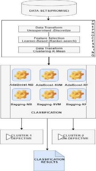
Fig.1. Hybrid ensemble learning approach.

_ max(y_n)-min(y_n)

к

yields the following cuts in the intervals:

min(l4) + d,......., min(^) + (k - 1)d   (4)

“The equal width method assumes that the underlying data fits somewhat well into a uniform distribution. It is very sensitive to outliers and can perform extremely poorly under some conditions”.

3.3 Feature Selection

The selection of features is the most critical stage in the construction of hybrid models for software defect prediction and for improving the efficiency of data mining algorithms. Ultimately, classifier input data is in a high-dimensional feature space, but not all features apply to the classes to be categorized, and some of the data includes features that are irrelevant, redundant, or noisy. In this case, noisy data can be introduced by irrelevant and redundant features that distract the learning algorithm. Feature Selection reduces the number of attributes; eliminates irrelevant, noisy, or redundant features; and effects applications by speeding up algorithms for data mining. Feature selection increases

the rate of identification and reduces the false alarm rate in software defect prediction.

A machine learning tool called WEKA 3.7. was used to measure the ensemble classifier selection features to check the classification quality of each of the feature sets. The ClassifierAttributeEval and Ranker algorithms were used to pick specific features from the dataset and to eliminate the features that were irrelevant before the clustering and classification. For this function, the whole training dataset and 10-fold cross-validation was used. The dataset was classified into 10 sub-datasets and the above algorithms were applied to them all.

• 3.4 K-mean

K-mean clustering is an unsupervised solution and used for hybrid ensemble learning methodology of training datasets. The cluster centers are determined after the initial random assignment of a sample to the clusters with the nearest centers. The process is repeated until there is no significant change in the cluster centers. The mean distance of the component to the cluster centers is used as the score when the cluster assignment is set. A set of Xj vectors in which j = (1,..., n) was divided into Gi groups in C, where I = (1,..., c). In the following formula, the function centered on the Euclidean distance between the Xj vector in group J and the corresponding Ci cluster center

7 = E^oZ/E^dЕк^с^И^ - С/П2] (5)

• IV.    Performance Prediction Matrices

Various software defect prediction measurements were addressed, such as true positive (TP), true negative (TN), false positive (FP), and false-negative (FN): “TP represents the number of defective instances of software that are correctly classified as defective, while TN is the number of instances of clean software that are accurately classified as correct. FP denotes the number of instances of clean software that are wrongly classified as defective and FN denotes the number of instances of defective software that are wrongly classified as clean [13]". The matrices used for the software defect prediction are shown in Table 1. Classification accuracy is one of the primary simple metrics for assessing the performance of predictive models and is often called the right classification rate.

Table 1. Threshold metrics for classification evaluations [27].

Metrics	Formula	Evaluation Focus
Accuracy	t p + t n t p + f p + tn + f n	“In general, the accuracy metric measures the ration of correct predictions over the total number of instances evaluated.”
Error Rate	f p +f n t p + f p + t n + f n	“Misclassification error measures the ratio of incorrect predictions over the total number of instances evaluated.”
Sensitivity	t p t p + f n	“This metrics is used for the fraction of positive patterns that are correctly classified.”
Specificity	t n t p + f p	“This metric is used to measure the fraction of negative patterns that are correctly classified.”
Recall	t p t p + f p	“Recall is used to measure the fraction of positive patterns that are correctly classified.”
F-measure	2 *p*r p + r	“This metric is Hormonic mean of Precision and recall.”
Geometric mean	^n * t p	“This metric is maximizing the tp and t n rates.”
Average Accuracy	L У      t p/ + t n/ ^ t p/ + f pi + t ni + f ni	“The average Effectiveness of all classes.”
Average Error Rate	У      f pt + f nt t p/ + f p/ + t n/ + f n/	“The average error rate of all classes.”
Average Precision	у   t p/ t p/ + f p/	“The average of per class precision.”
Average Recall	у   t p/ t p/ + f n/	“The average of per class recall.”
Average F-measure	2*Pm*Pn P m + P n	“Average of per class f-measure.”
Note: Where t p is true positive rate for class C / , t n/ is true negative rate for class C / , f n/ is false negative rate for class C / , and fp / is false positive rate for class C / .

• V.    Experimental Study

• 5.1    Performance analysis of HELT

“Table 2 provides a brief description of the PROMISE datasets used in this analysis [29]. The attributes of these datasets are presented in Table 3”.

Table 2. Datasets from PROMISE repository.

No	Dataset	Module	Defective module	Non-defective module	Defective	Class imbalance rate
					Non-defective
1.	CM1	327	45	282	0.159	11.9
2.	JM1	7782	1672	6110	0.274	21.5
3.	KC3	194	36	158	0.228	18.6
4.	MC1	1988	46	1942	0.024	2.3
5.	MC2	125	44	81	0.543	35.2
6.	PC1	705	61	644	0.095	8.7
7.	PC2	745	16	729	0.022	2.1
8,	PC3	1077	134	943	0.142	12.4

Table 3. PROMISE software defect prediction attribute details.

Attribute Information :

1. loc:	numeric McCabe's line count of code
2. v(g):	numeric McCabe "cyclomatic complexity"
3.    ev(g) 4.    iv(g):	numeric McCabe "essential complexity" numeric McCabe "design complexity"
5. n	numeric Halstead total operators + operands
6. v	numeric Halstead "volume"
7. l	numeric Halstead "program length"
8. d	numeric Halstead "difficulty"
9. i	numeric Halstead "intelligence"
10. e	numeric Halstead "effort"
11. b	numeric Halstead
12. t	numeric Halstead's time estimator
13. lOCode	numeric Halstead's line count
14. lOComment	numeric Halstead's count of lines of comments
15. lOBlank	numeric Halstead's count of blank lines
16. lOCodeAndComment:	numeric
17.    uniq_Op 18.    uniq_Opnd 19.    total_Op 20.    total_Opnd 21: branchCount	numeric unique operators numeric unique operands numeric total operators numeric total operands numeric of the flow graph
22. defects	{false,true} module has/has not one or more reported defects

Weka [28] was used to build a model based on hybrid algorithms called HELTs in Java. The datasets were split into 10 consecutive folds to conduct 10-fold crossvalidation. One part for testing and the other for training folds. Using the standard Scaler method in Weka, the features were then standardized and scaled. The performance of the HELT is presented in Tables 4–7, and the calculation of the MLT is given in Table 8.

As shown in Table 2, the dataset was very imbalanced. Therefore, we used the oversampling technique SMOTE to make balance it. The comparative results indicate that performance improved in all datasets after applying the hybrid methodology (see Figures 2 and 3). As shown in Table 4, the performance of the AdaBoost SVM and the bagging SVM was very high for some datasets, while the AdaBoost RF and the bagging RF achieved 100 for dataset JM1. It became possible when we used for feature selection ClassifierAttributeEval, Ranker as a search method and K-mean for data Transformation.

Table 4. HELT accuracy .

	AdaBoost NB	AdaBoost SVM	AdaBoost RF	Bagging NB	Bagging SVM	Bagging RF
CM1	89.6	94.49	90.51	78.89	92.66	90.82
JM1	99.84	100	100	99.75	100	100
KC3	94.44	96.29	95.3	96.29	96.29	95.83
MC1	99.2	99.8	99.7	98.55	99.65	99.6
MC2	98.26	97.68	98.84	97.6	98.26	98.26
PC1	98.08	98.22	98.77	98.08	98.49	98.63
PC2	93.26	100	90.47	84.87	100	90.47
PC3	91.32	100	88.85	82.28	100	88.58

Table 5. HELT F-measure .

	AdaBoost NB	AdaBoost SVM	AdaBoost RF	Bagging NB	Bagging SVM	Bagging RF
CM1	89.6	94.5	90.05	78.1	92.6	90.8
JM1	99.8	100	100	99.8	100	100
KC3	94.5	96.3	95.4	96.3	96.3	95.9
MC1	99.2	98.8	99.7	98.6	99.7	99.6
MC2	98.3	97.7	98.9	97.7	98.3	98.3
PC1	98.1	98.2	98.8	98.4	98.5	98.6
PC2	93.2	100	90.2	85.2	100	90.2
PC3	91.3	100	88.9	82.3	100	88.6

Table 6. HELT AUC .

	AdaBoost NB	AdaBoost SVM	AdaBoost RF	Bagging NB	Bagging SVM	Bagging RF
CM1	94.5	93.8	96.3	91.3	97.7	96
JM1	100	100	1OO	99.6	100	100
KC3	97.7	96.3	98.3	98.8	98.3	98.6
MC1	99.9	99.6	100	99.3	100	100
MC2	99.6	97.8	99.7	99.8	99.5	99.5
PC1	99.7	94.8	99.8	99.7	99.8	99.8
PC2	93.2	100	97.4	92.7	100	97.3
PC3	97.4	100	95.9	90.2	100	95.9

Table 7. HELT recall .

	AdaBoost NB	AdaBoost SVM	AdaBoost RF	Bagging NB	Bagging SVM	Bagging RF
CM1	89.6	94.5	90.05	78.9	92.7	90.8
JM1	99.8	100	100	99.8	100	100
KC3	94.4	96.3	95.4	96.3	96.3	95.8
MC1	99.2	99.8	99.7	98.6	99.7	99.6
MC2	98.3	97.7	98.9	97.7	98.3	98.3
PC1	98.1	98.2	98.8	98.4	98.5	98.6
PC2	93.3	100	90.5	85.2	100	90.5
PC3	91.3	100	88.9	82.3	100	88.6

Table 8. Accuracy MLT .

	NB	SVM	RF
CM1	78.89	92.94	89.5
JM1	94.98	95	96.11
KC3	91.29	92	92.81
MC1	93.9	97.98	94.44
MC2	92.69	95.52	93.54
PC1	92.67	93.61	92.81
PC2	79.37	94.44	88.5
PC3	82.28	93.99	89.1

Figure 2 : Accuracy MLT and Accuracy HELT for Naive Bayes

CM1     JM1     KC3     MC1    MC2     PC1     PC2     PC3

—е—NB  —•—ADABOOST-NB  —•—BAGGING-NB

• Fig. 2.    MLT and HELT accuracy for Naive Bayes.

Figure 3 : Accuracy MLT and Accuracy HELT for SVM

CM1     JM1     KC3     MC1    MC2     PC1     PC2     PC3

—•—SVM  —•—ADABOOST-SVM  —•—BAGGING-SVM

• Fig. 3.    MLT and HELT accuracy for SVM.

  
  

  Figure 4 : Accuracy MLT and Accuracy HELT for RF

  
  
  

CM1     JM1     KC3     MC1    MC2     PC1     PC2     PC3

—•— RF  —е—ADABOOST-RF  —•—BAGGING-RF

• Fig. 4.    MLT and HELT accuracy for RF.

• VI. Paired T-Tests

For this purpose “The hypotheses can be formulated in two different ways, expressing the same concept and being identical mathematically [30]”: we uses SPSS for paired T-test. Here we uses the accuracy, F-measure and recall on all dataset to check the hypothesis is rejected.

“ H 0 : µ 1 = µ 2 : In terms of their ability to predict defects, different methods used in the analysis are statistically similar”.

“ H 1 : µ 1 ≠ µ 2 : In terms of their ability to predict defects, different methods used in the analysis are statistically different”.

where

• 1.    “µ 1 is the population means of Algorithm 1, and

• 2.    µ 2 is the population means of Algorithm 2”.

  Table 9. Paired t-test results.

  		Paired Differences					t	df	P-Value
  		Mean	Std. Deviation	Std. Error Mean	95 Confidence Interval of the Difference
  					Lower	Upper
  Pair 1	AdaBoostNB -AdaBoostSVM	-2.81	3.498	1.23	-5.73	0.114	-2.27	7	0.067
  Pair 2	AdaBoostNB -AdaBoostRF	0.195	1.523	0.53	-1.078	1.468	0.36	7	0.728
  Pair 3	AdaBoostNB -BaggingNB	3.461	5.003	1.76	-0.72	7.644	1.95	7	0.091
  Pair 4	AdaBoostNB -BaggingSVM	-2.668	3.316	1.17	-5.44	0.103	-2.27	7	0.057
  Pair 5	AdaBoostNB -BaggingRF	0.226	1.638	0.57	-1.14	1.596	0.39	7	0.708
  Pair 6	AdaBoostSVM -AdaBoostRF	3.00	4.801	1.69	-1.01	7.019	1.77	7	0.120
  Pair 7	AdaBoostSVM -BaggingSVM	0.14	0.719	0.25	-0.46	0.742	0.55	7	0.596
  Pair 8	AdaBoostSVM -BaggingRF	3.03	4.806	1.69	-0.98	7.054	1.78	7	0.117
  Pair 9	AdaBoostRF -BaggingNB	3.26	4.28	1.51	-0.32	6.849	2.15	7	0.068
  Pair 10	AdaBoostRF -BaggingRF	0.03	0.33	0.12	-0.25	0.315	0.26	7	0.802
  Pair 11	BaggingNB -BaggingSVM	-6.13	7.87	2.78	0.320	0.451	-2.20	7	0.063
  Pair 12	BaggingNB -BaggingRF	-3.23	4.33	1.53	-6.86	0.392	-2.10	7	0.073
  Pair 13	BaggingSVM -BaggingRF	2.89	4.74	1.68	-1.07	6.864	1.72	7	0.128

  
  

As all the p-values are greater than the significance level (0.05, the null hypothesis is accepted. Consequently, the performances of various techniques used for predicting defects are statistically identical, i.e. the HELT performance is equally effective for all datasets.

• VII. Answers To The Research Questions

The answers to different study questions are the following:

Q1 . How well does the HELT predict software defects using the change of metrics?

Answer : In all four HELTs used for software defect prediction, the performance of AdaBoost SVM and bagging SVM was best in terms of accuracy, recall precision, and AUC.

Q2 . How HELT is better than existing machine learning techniques (MLTs) for software defect prediction?

Answer : A high accuracy rate was shown by HELT vs. MLT based on the software defect prediction model.

Q3 . Are the available techniques in discussion hypothetically equal?

Answer : The null hypothesis was accepted for the accuracy of the techniques, therefore, there is no statistical difference between the performances of different algorithms.

• VIII.    Threats To Validity

As an open-source NASA repository based on java was used, so there is a chance of threat to generalize results for other languages like Python, R programming, etc. The size of the dataset may also affect the probability of the class being defective, and the dataset collection may not be representative. The latter is mitigated in our analysis by testing the classifier output on eight well-known datasets that have been widely used in the previous literature. “The optimization algorithms may over-fit and bias the results. Instead of randomly splitting the datasets using the simple train test split (20–30 for testing and 70–80 for training), we split the dataset into training and test sets using 10-fold cross-validation to prevent the over-fitting problem that could be triggered by random splitting”.

• IX.    Conclusion

This study compared the results of different machine learning algorithms with hybrid ensemble learning for software defect prediction. As it is effective at reducing testing efforts, the identification of defective classes in software has been considered. Scientific data were used to predict the software's future release, and classification accuracy F-measurements and ROC-AUC metrics were used to test the performance of various algorithms. To improve the data balance, the SMOTE method was used.

The results of the study showed that the performance of HELT with AdaBoost SVM, AdaBoost RF, and bagging SVM gives the best results in accuracy recall, AUC and F-measure, with up to 100 accuracy. Future studies should explore and compare the performance of Artificial Neural Networks approaches and Hybrid ensemble classifiers with other oversampling methods as data imbalance has a significant impact on the performance of the current software defect prediction approaches.