Hyperspectral image segmentation using dimensionality reduction and classical segmentation approaches

A hyperspectral image is a three-dimensional array having two spatial dimensions, and one spectral dimension. Every pixel of a hyperspectral image is a vector containing hundreds of components corresponding to a wide range of wavelengths. Compared to grayscale and multispectral images, hyperspectral images offer new opportunities allowing to extract information about materials (components) located on images. Thanks to these unique properties, hyperspectral images are used in agriculture, medicine, chemistry and many other fields.

However, high dimensionality of hyperspectral images often makes it impossible to directly apply traditional image analysis techniques to such images. For this reason, hyperspectral image analysis became an extensively studying area last years. In this paper, we consider the segmentation of hyperspectral images, which is one of the most important tasks in hyperspectral image analysis [1 - 6]. Other important tasks include, for example, classification [7], detection of anomalies [8], etc.

Image segmentation is the process of partitioning an image into connected regions with homogenous properties. In image analysis, segmentation methods are usually divided into three classes [1]: feature-based methods, region-based methods, and edge-based methods.

Feature-based methods split all image pixels into subsets, based on their values or derived properties. Thus, first class of methods operates in spectral or derived space. This class includes methods based on clustering [2, 3]. Region-based and edge-based methods operate on a spatial domain. Region-based methods use some homogeneity criterion to detect regions in an image. This class includes methods based on region growing, and watershed transformation [4, 5]. Edge-based methods use the properties of discontinuity to detect edges, which split an image into regions. Methods belonging to the last class are used quite rare with hyper- spectral images due to the ambiguity in detecting edges in hyperspectral images.

There are a growing number of papers that use both unsupervised segmentation and supervised classification techniques to build sophisticated classification methods with improved classification accuracy [5, 6, 19].

It should be noted, sometimes in literature, segmentation methods are also divided into two classes: unsupervised and supervised methods. To avoid confusion, in this paper we will consider segmentation as an unsupervised procedure. Thus, we refer a supervised segmentation as a classification task.

Despite the fact that there are a lot of papers devoted to the development of new segmentation methods, and improvement of classification techniques, there is a lack of papers containing the evaluation of well-known classical segmentation approaches for hyperspectral images. Moreover existing papers on unsupervised segmentation often do not introduce any numerical measure to evaluate and compare methods, contenting with a qualitative assessment. In this paper, to partially fill this gap, we follow the straightforward approach reducing the dimensionality of a hyperspectral space, and evaluating three classical segmentation techniques. These techniques are clustering technique, region-growing technique, and watershed transform.

The paper is organized as follows. Section 1 introduces the general segmentation scheme used in this paper. Particular components of the scheme including segmentation approaches and the assessment of the segmentation quality are described in Section 2. Section 3 contains the experimental results and discussion. The paper ends with conclusions followed by References and Appendix sections.

1.    General segmentation scheme

This study follows the general segmentation scheme depicted in the Fig. 1.

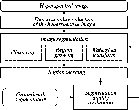
Fig. 1. General segmentation scheme.

Alternative methods are shown with dash-dot lines, optional elements are shown with dash line

According to the above scheme, there are four consequent stages. At the first stage, the spectral dimensionality of a source image is reduced using the principal component analysis technique, which is the most well-known and widely used linear dimensionality reduction technique. At the second stage, an image is segmented using one of the classical segmentation techniques. Here each segmentation method takes a set of possible parameters and produce a set of segmented images. This allows further to determine suboptimal parameters for each of the segmentation methods. At the third stage, an optional region merging procedure is involved. It is supposed that this procedure can improve segmentation quality for oversegmented images by merging adjacent regions with similar features. In any case, the quality of all the segmented images is evaluated automatically at the last stage. To accomplish this, we provide groundtruth segmentation images to the evaluation procedure.

2.    Methods

Dimensionality reduction

To reduce the dimensionality of hyperspectral data both linear and nonlinear dimensionality reduction techniques are used. Linear techniques including principal component analysis (PCA) [9], independent component analysis (ICA) [10], and projection pursuit are used more often. Nonlinear dimensionality reduction techniques (nonlinear mapping [11, 12], Isomap [13], locally linear embedding [14], laplacian eigenmaps [15]) are used less often due to the high computational complexity of such techniques.

In this paper we adopt the PCA technique as this is the common choice in such cases. This technique finds linear projection to a lower dimensional subspace maximizing the variation of data. PCA is often thought of as a linear dimensionality reduction technique minimizing the information loss. In this paper we use PCA to project hy-perspectral data to low-dimensional space.

The following Fig. 2 shows a hyperspectral image used in this paper to conduct experimental study. The image in pseudo colors is produced by the reduction of a hyperspec-tral space to a 3D space using the PCA technique followed

c)

by the projection of the reduced space into the RGB color space so that the first principal component corresponds to the green color, the second principal component – to the red color, and the third component – to the blue color.

a)

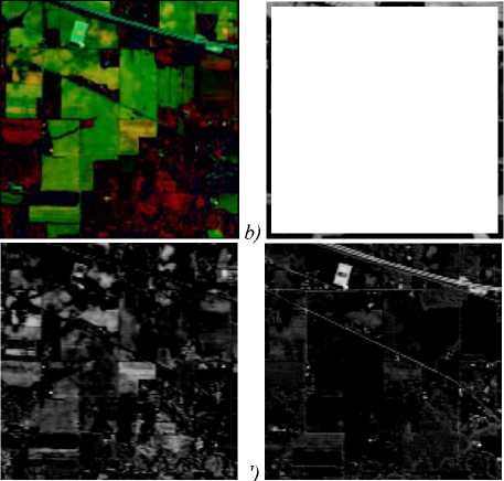
false color image produced using projection of first three principal components into green, red, blue channels of the RGB color space (a), color figure online; and the first, second and third principal components, contrasted (b-d)

d)

Fig. 2. Indian Pines Test Site 3 hyperspectral scene:

Clustering technique

A segmentation method based on a clustering technique is quite straightforward. It consists of two steps. At first, a clustering of image pixels is performed in a reduced space. At this stage, a clustering algorithm partitions a set of image pixels into some number of subsets, according to pixels features. At the second stage, an image markup procedure extracts connected regions of an image containing pixels of corresponding clusters.

There is a number of clustering algorithms belonging to the following classes [3]: hierarchical clustering, density-based clustering, spectral clustering, etc. While a number of clustering algorithms have been proposed, the well-known k-means algorithm [16] remains the most frequently mentioned approach. In this paper, we used this algorithm with the squared Euclidean distance measure. To initialize cluster centers we used the k-means++ algorithm [17, 19]. It was shown that k-means++ algorithm achieves faster convergence to a lower local minimum than the base algorithm.

To obtain a satisfactory solution, we varied the number of clusters from 10 to 100. For each specified number of clusters we initialized and ran clustering for 5 times to get the best arrangement out of initializations.

Thus, the standard clustering approach can be expanded for hyperspectral image processing in a natural way. This is ensured by the ability of clustering algorithms to work in high-dimensional spaces. So the key issues here are the quality of clustering in a hyperspectral space, and the time of processing, as a clustering is a time consuming procedure.

Region growing

The main idea of a region growing approach consists in growing regions, starting with the selected set of so-called seed points. This approach consists of two stages. At the first stage, seeds are selected using some algorithm. At the second stage, the regions are grown from the selected seeds. At this stage, some homogeneity criterion is used to check whether adjacent pixels belong to the growing region or not.

A selection of seed points is an important issue of the considered approach. In this paper we select local minimums of the absolute value of a gradient image as seed points (see Watershed transform section for more details on a gradient image). Besides that we used simple homogeneity criterion based on Euclidean distance between examined pixels and corresponding seeds. Thus, the segmentation method, which is based on the region growing approach, has one tunable parameter (threshold) used in the homogeneity criterion.

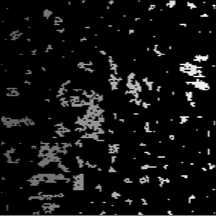
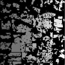
The following Fig. 3 shows different stages of the algorithm. The number of seeds in this example was reduced by applying morphological operations (opening and closing) to the gradient image. Another issue related to the region growing technique is the dependency of the resultant segmentation on the order of seeds (in the Fig. 3 the darker regions are processed prior to the brighter ones).

To segment an image using watershed transform, we start with searching of the local minima of the gradient of an image. Then we apply the watershed transform to obtain the boundaries of regions. Having boundaries, we use an image markup procedure that extracts connected regions inside boundaries. Finally, we classify each boundary pixel to one of the adjacent regions using nearest neighbor rule.

The main issue of the watershed transform for hyper-spectral images consists in gradient computation. There are two different approaches [5] to gradient computation: multidimensional and vectorial gradient computation. In our preliminary experiments we used both approaches. In particular, we implemented metric-based gradient [4] belonging to the vectorial gradient, and several multidimensional gradients based on aggregation [5] of onedimensional gradients using summation, maximum or L2 norm operators. Other possible solutions such as combination of watershed segmentations of individual channels of a hyperspectral image were not considered.

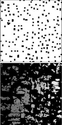
Fig. 3. Region growing: seeds map (a) and regions with different growing threshold parameters (b-d)

a)

b)

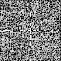
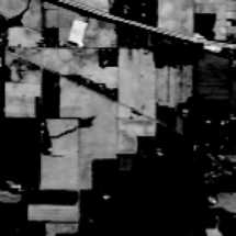
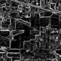
Fig. 4. Watershed transform: gradient image (a); watershed map (b)

d)

Watershed transformation

A watershed transform [18] considers a grayscale image as a topographic relief. We place water sources in each local minimum (pixel with locally minimal value on a height map). That is, water sources are located at the bottom points of so-called catchment basins. Than we flood catchment basins with water from sources. We place boundaries at image pixels, where different water sources meet.

Region merging procedure

Unfortunately, each of the considered segmentation approaches can produce an over-segmented image according to the following reasons:

• -    an excessive number of clusters in the first approach,

• -    an excessive number of local minima in a gradient image in the second and third approach.

To overcome the problem of over-segmentation we use an optional region merging stage (according to the Fig. 1). The main idea of the merging procedure is to merge adjacent regions with similar characteristics, starting with the most similar regions. A brief description of the merging procedure is given below.

At first, we form the list of adjacent regions, which contains information on all unique pairs of adjacent regions. At second, we calculate the similarity of regions for each pair in the list. After that we put all extracted pairs into a priority queue so that pairs of similar regions have higher priority in the queue. Finally, we iteratively exclude pairs with highest priority from the queue, merge corresponding regions of an image, and update information in the queue. A stopping criterion here can be based on a number of regions or on a merge threshold. In this work we used the latter case based on a tunable threshold parameter.

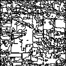
Fig. 5. Boundaries of segments obtained after region merging procedure for the example shown in the Fig. 2

Segmentation quality evaluation

A large number of segmentation quality evaluation measures have been developed by researchers. These measures can be divided [23] into several classes: regionbased quality evaluation measures (taking into account the characteristics of the segmented regions), edge-based quality evaluation measures (taking into account the characteristics of boundaries of the segmented regions), measures based on information theory, and nonparametric measures. The first class includes the so-called directional Hamming distance [20], which is asymmetrical measure, and normalized Hamming distance [20], Local / global consistency errors [23], etc. The second class includes the precision and recall measures [21], earth movers distance [22], and others. An example of the third class is the variation of information [26]. The fourth class includes the Rand index [24], its variations, and some other measures.

In spite of the large number of developed evaluation measures, there is a lack of papers devoted to the comparative analysis of such measures [25]. This complicates the clear choice to any particular measure of the segmentation quality. Given the fact that the study of measures of segmentation quality is not the main purpose of this work, in this paper we use the consistency errors [23] and Rand index [24] as one of the most commonly used measures.

Global Consistency Error [23] is expressed by the formulae:

GCE ( S i , S 2 ) = Imin{^ i ( S 1 , S 2 ), ^ 8 , .( S 2 , S i ) } .

Here S 1 and S 2 are two segmentation results to be compared, N is the number of pixels in an image and

8 , ( S 1 , S 2 ) =

^{| R} 1 i ^{\ R} 2 i ^|

^{| R} 1 i ^|

is a measure of error for the i-th pixel, R 1i is a region containing i-th pixel on S 1 segmentation, R 2i is a region containing i-th pixel on S 2 segmentation.

As an alternative evaluation approach, we use the Rand Index (RI) [24] to estimate the quality of segmentation.

RI ( S 1 , S 2 ) =       X ( I ( l , ¹ = l> l 2 = l 2 ) +

I ^ I i ■ j

I 2 J ‘ * j

+ 1 ( l i * l ‘ л l , ² * l j ² ).

Here I () is the identity function, l_i ^k is the label (segment) of the i -th pixel on the k -th segmentation. The denominator is the number of all possible unique pairs of N pixels.

It is worth noting, that the above measures do not directly reflect the quality of classification. Nevertheless we use them here as we consider segmentation as an unsupervised procedure.

3.    Experimental results

In this section we describe the results of the experimental study according to the general scheme described in the second section.

In our experiments, we used open and well-known hyperspectral remote sensing scenes [27]. Here we provide experimental results for Indian Pines scene, which was acquired using AVIRIS sensor (some results for the Salinas hyperspectral scene are present in the Appendix). Indian Pines image contains 145×145 pixels in 224 spectral bands. Only 200 bands were selected by removing bands with the high level of noise and water absorption. This hyperspectral scene is provided with the groundtruth segmentation mask that is used to evaluate the quality of segmentation (Fig. 6).

Segmentation quality

The results of the quality evaluation for the k-means clustering technique are shown in the Fig. 7. Fig. 7 a shows the dependency of the clustering quality on the dimensionality of the reduced space. Here we use the following quality measure:

5 = -^^L" XI C J

k = 1

K

■H d 2( x, Ck ), k=1 x, e Ck where K is the number of clusters, |Ck| is the number of pixels in the cluster Ck, d(xi, ck) is the Euclidean distance between pixel xi and the centroid ck of the cluster Ck measured in the source hyperspectral space.

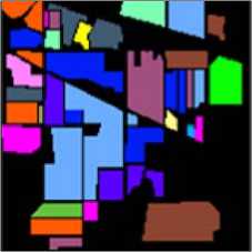
Fig. 6. Groundtruth classification of the Indian Pines Test Site 3 hyperspectral scene (color figure online)

As it can be seen from the Fig. 7 a the error of clustering decrease rapidly with the first few dimensions, and then remains almost unchanged. This allows us to suggest that, for the considered clustering technique, we can perform segmentation in relatively low dimensional spaces without deterioration of the segmentation quality. This assumption is supported by the results of further evaluation of segmentation quality.

An example of the segmentation quality evaluation for the clustering based approach is shown in the Fig. 7 b .

Clustering error

0.0370 At

0.0365 -I

0.0360 [

0.0355-'^

0.0350 "

a) 0

k-means, К=20

dim

Segmentation evaluation 0.15 -i GCE

0.10-,

RI

0.05-

.GCE

0 I—

b) 10

150    200

к-means, dim=5 RI г 0.90

-0.89

--0.88

-0.87

-0.86

---Г-- 0.85

Fig. 7. Segmentation evaluation for the k-means ++ clustering algorithm: the dependency of clustering quality on the dimensionality (a); the dependency of the segmentation quality on the grow threshold parameter for a fixed dimensionality (b)

It should be noted that lower values of the GCE measure are better than the higher ones. Conversely, for the RI measure, higher values are better. As it can be seen from the figure both measures decrease monotonically with increasing number of clusters. It means that the GCE measure improves with the number of clusters, but the RI measure deteriorates simultaneously. In such situation, one could restrict the loss of one measure, and optimize another one.

Experimental results for the algorithms based on the region growing approach and watershed transform are shown in a Fig. 8, 9 correspondingly. As it can be seen from the figures, the threshold parameter allows to fine tune the quality of the segmentation. In the case of the region growing algorithm and in the case of the watershed transform as well, both indicators behave in the opposite way achieving their best values at approximately the same parameter values.

Segmentation evaluation Region growing, dim=5

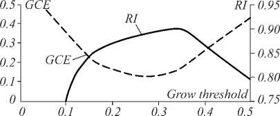
Fig. 8. Segmentation evaluation for the region growing algorithm. The dependency of quality measures on the growth threshold parameter for a fixed dimensionality

As in the case of the k-means++ algorithm, we cannot point to any significant dependency of the segmentation quality on the dimensionality of the reduced space.

Tables 1 and 2 (see Appendix) summarize best values of the quality measures. In these tables, we restrict the loss of one measure, and optimize another one. In Table 1 we restrict the descent of the RI measure by values 0.88 (less strict case), and 0.885 (more strict case), and search for the best (lower) values of the GCE measure. In Table

2 we restrict the growth of the GCE measure by values 0.2 (less strict case), and 0.15 (more strict case) and search for the best (higher) values of RI.

Segmentation evaluation          Watershed, dim=3

0.5_л GCE                             RI г 0.95

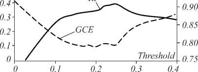
Fig. 9. Segmentation evaluation for the algorithm based on the watershed transform. The dependency of quality measures on the threshold value for a fixed dimensionality

As it can be seen from the results of the experiments, best values of the GCE measure are provided by the k-means segmentation approach. Best values of the RI measure are provided by the region growing approach. The watershed transform often takes up an intermediate position.

Some segmentation examples for all the considered techniques and different parameters are provided in Table 5 in Appendix.

Tables 3 and 4 (see Appendix) present some results of the experimental study for the Salinas [27] hyperspectral image. The Salinas image also was acquired by the AVIRIS sensor. This image contains 217×512 pixels and the same number of spectral bands. As in the previous case, we used corrected image, which contains 204 spectral bands. As in the previous case, Table 3 contains best (lower) values of the GCE measure with restriction on the RI measure. Table 4 contains best (greater) values of the RI measure with restriction on the GCE measure. As it can be seen from the considered tables, the experiments confirmed the described above results for the Indian Pines image.

Time evaluation

In this section we estimate the time of processing for each considered approach. It is worth noting that all the evaluated techniques were implemented as test scenarios using Matlab, and final timings may vary on the details of implementation, environment and hardware.

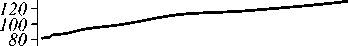
The results of the evaluation are shown in Fig. 10. As it can be seen, the dimensionality reduction stage (Fig. 10 a ) takes much less time compared to segmentation algorithms (Fig. 10 b - d ). Timings for all three segmentation techniques grow almost linear with the dimensionality. It is consistent with the theoretical estimations as for the k-means and region growing approaches it is necessary to calculate dissimilarities (distances) between vectors in a reduced space, and each calculation requires O[dim] operations. For the watershed transform it is required to aggregate gradient images. This also requires O[dim] operations.

Overall, it is possible to significantly speed up the segmentation procedure without quality loss by reducing the dimensionality of hyperspectral images, if the k-means++ or the region growing segmentation is used. The use of dimensionality reduction stage does not give visible advantages to the segmentation technique based on watershed transformation.

Dimensionality reduction time PCA

• 1 .00 ч t

0.08----------------------------- 0.06 0.04 0.02-,

________________________

• a) 0         50      100     150200

Segmentation time к-means, K=20

150 ч t

b) 0         50      100     150200

Segmentation time Region growing, 140ч t                            ^,=03

________________________

c) 0         50      100      150200

Segmentation time 3.0ч t

Watershed transform

2.5

2.0

1.5

1.0

0.5

d) 0

50      100     150    200

Fig. 10. Time evaluation. The dependency of time

(in seconds) on the dimensionality:

for PCA based dimensionality reduction (a);

for k-means++ based segmentation (b);

for region growing segmentation (c);

for watershed transform based segmentation (d)

Conclusion

In this work, we evaluated several classical image segmentation techniques in the task of segmenting hyperspec-tral remote sensing images. These techniques are the k-means clustering approach, region growing technique, and technique, based on the watershed transform. To perform the evaluation we reduced the dimensionality of the hyperspec-tral data, performed segmentation, and then evaluated the quality of segmented images. Experimental study showed that best values of the GCE measure were provided by the k-means segmentation approach. Best values of the RI measure were provided by the region growing approach. The watershed transform takes up an intermediate position.

Besides, it was shown that it is possible to significantly speed up the segmentation procedure without substantially quality loss by reducing the dimensionality of hyperspectral images, if k-means++ or region growing segmentation is used. Therefore, the considered approach can be useful in semi-automatic hyperspectral image analysis tools.

In the future, we plan to study nonlinear dimensionality reduction techniques based on different spectral dissimilarity measures as a prior step to hyperspectral image segmentation.