Image Classification Using Fusion of Holistic Visual Descriptions

In the recent years, advancements in technology have made procurement of multimedia content easier than ever before. The use of World Wide Web has made it possible to exchange acquired content throughout the world, thus multiplying the amount of data available and accessible. Multimedia data consists of various media types such as text, images, audio, video sequences and animation. Advanced and readily available methods of image acquisition have led to the creation of a variety of digital images such as of a physical scene or the interior tissue structure of an organ. This implausible growth results in the generation of very large and detailed image databases which necessitates the development of intelligent systems to understand such large, complex, information-rich data sets. Computer vision is a field of study which combines different methods for acquiring, processing, analyzing and understanding images. Image mining is a heterogeneous research area which embraces a large spectrum of methods from computer vision, image processing, image acquisition, image retrieval, data mining, and machine learning. It essentially deals with extracting inherent patterns from collection of images [1].

Content based image mining consists of various data mining tasks which exploit image content based features to discover knowledge from a collection of images. The outcome of different mining tasks (classification, clustering or generation of association rules) may vary from one application domain to another. For example in [13] a study of area of land use and land cover change analysis based on satellite images is presented. In the domain of medical diagnosis an image mining system may utilize the results of clinical reports (textual data) along with the content of images in the form of X-ray or CT scan image to predict a disease. Similarly, images can be clustered into groups based on their content such as similar color or shape which can find application in content based image retrieval.

This paper addresses the task of scene understanding and development of a system which can efficiently perceive, process, and understand visual data in scene images. The aim of our work is efficient classification of scene images into appropriate category using machine learning and computer vision techniques. Regarding scene perception two types of cognitive approaches are used. The first is an object-centered approach which describes a scene in terms of the objects contained in it and the second is the scene-centered approach which does not rely on the occurrence of objects.

Our work is essentially scene centered and the purpose is to provide a “holistic” description of a scene using low level visual cues and assign it to its category such as sunrise/sunset, beach, highway, waterfalls or to be a basic block in computer vision based expert systems. We have chosen this approach since it closely resembles human perception of scenes. A quick visual perception does not heavily rely on the recognition of objects and detailed information. The presence of certain kind of objects is deduced even though it is not necessary that each object is recognized. The global image features can be used to assess the composition of a scene thus serving as an aid to rapid scene recognition.

Scene classification is useful in applications such as content-based image organization and context-sensitive management of images. The primary contributions of this paper are two-fold. Firstly to evaluate how the global features could contribute to real-world scene categorization, we extract appropriate low-level features and use early fusion to find the best combination of state-of-the-art computer vision features. Secondly, we analyze two different classifiers using cross-validation procedures for scene classification.

The rest of the paper is organized as follows: Section 2 presents the motivation behind present work. Section 3 gives a brief overview of previous work in scene categorization using low level descriptions. Section 4 presents the different kinds of image descriptors used in this paper as well as description of the data set used. It also elaborates the feature fusion technique and classifiers used. Section 5 presents experimental results. Section 6 presents detailed result analysis. Section 7 presents the advantages of our approach. Finally, Section 8 draws the conclusions and future directions.

• II.    Motivation

With advancements in technology the multitude of images generated every day necessitates their categorization, organization and retrieval in a fast and efficient way. For example a family on a vacation trip may capture images of coastal areas, skyscrapers, mountains and waterfalls. Automatic categorization of such scenes would help in effective management and access. Thus scene classification into semantic categories (e.g. coast, mountains and streets), is a challenging problem nowadays. The major approaches to scene classification are based on low level-features or semantic features. The motivation behind our work is find the answer to the question “Is it possible to capture the gist of the scene using a low-dimensional signature (feature) vector?”Although there is semantic gap between low-level features and high- level concepts, but effective low-level discriminating features which provide holistic scene understanding information may be used to derive middle level and symbolic and/or semantic features.

• III.    Literature Review

Psychophysical and psychological studies have shown that scene identification by humans can proceed, in certain cases, without any kind of object identification suggesting the possibility of coarse scene identification from global low-level features [11], [12]. A number of research studies have attempted to derive high level image semantics from low level features. This section presents notable contributions in this area. Szummer and Picard [9] and Yiu [10] propose algorithms for indoor outdoor scene classification. Yiu uses color and dominant directions for image classification over a dataset of 500 images. Szummer and Picard have proposed color and texture features extracted over whole image as well as over 4x4 sub-blocks of images to perform classification over a dataset of 1343 images which depict typical family and vacation scenes including snow, bright sun, sea, sunset, night and, silhouette scenes. Initial contributions in the area of scene classification can be found in the works of Paek et al. [26], Savakis and Luo [27], Guerin-Dugue and Oliva [28] and N. Serrano, A. Savakis, J. Luo [29].

In [8] Vailaya et.al have considered the hierarchical classification of vacation images on a database of 6931 vacation photographs. For indoor/outdoor classification 10x10 sub-block color moments in LUV space; for city/landscape edge direction histograms and coherence vectors; for sunrise/sunset/mountain spatial moments, color histograms and coherence vectors in HSV/LUV space have been used. In [13] authors manually label each training image with a semantic label and train k classifiers (one for each semantic label) using support vector machines (SVM). Each test image is classified by the k classifiers and assigned a confidence score for the label that each classifier is attempting to predict. A k-nary label-vector consisting of k-class membership is generated for each image. The system is tested on 15 different scene categories. In the work of Oliva and Torralba [15] the scene structure is estimated by the means of global image features. The scene is described holistically by their degree of naturalness, openness ruggedness, expansiveness, etc. Spatial envelope representation using DST has been used to evaluate the spatial layout properties. The approach in [16] is used to classify and organize real-world scenes along broad semantic axes. Firstly, all the scenes are classified according to an Artificial to Natural axis. Then, natural scenes are organized along the Open to Closed axis whereas artificial environments are classified according to the Expanded to Enclosed scene’s axis. In [17] the authors represent the image of a scene by a collection of local regions, denoted as code words obtained by unsupervised learning. Each region is represented as part of a “theme”. The categorization is performed on a large set of 13 categories of complex scenes. Bosch et al. [18] use a probabilistic model to recognize the objects and classify the scene based on these object occurrences.

Several approaches using low level descriptors have been studied for scene classification. The authors in [20] describe scene images through multimodal features and explore the complementary characteristics of these features. A user labeling procedure has been introduced to reduce semantic gap. In [21] a multi-scale, statistical approach for representing images aimed at scene categorization is presented. At different levels, sets of features that represent exclusively the scene are selected. The non-characteristic elements such as foreground objects which do not contribute to scene classification are disregarded. Authors have obtained good results even with simple features like local color image histograms. In [22] authors have developed ARTSCENE: a neural system for classifying scenes. They assume that boundary, surface, and spatial information is combined to represent scene gist. The gist of a scene is represented by its spatial layout of colors and orientations. In our approach we aim at evaluating most discriminating color, texture features along with edge descriptors using two state of the art classifiers SVM and Neural Networks (NN). Features have been fused to find the best combination and classifier evaluation has been done using an exhaustive set of experiments; the SVM parameters have been derived using 10 fold cross validation.

• IV.    Materials and Methods

Any scene classification system must extract suitable features and use some learning mechanism to classify test or input images. This section outlines the individual features, the classifiers and dataset used in our experiments.

• A.    Image Descriptors

Feature extraction from images and selection of appropriate features is the key to the success of any image mining task [24]. The distinguishing low-level image features used in this paper are color, texture and edges.

Color

Human eye is more sensitive to color; therefore color acts as a discriminative feature for scene understanding applications particularly those which include outdoor images [23]. Color feature is robust to background complication and is independent of image size and orientation. For example a mountain scene can be characterized by blue sky on the top whereas a forest scene will contain large portions of green shades. The color features used are:

Color Moments

Color moments are scaling and rotation invariant and are based on the assumption that the color distribution in an image can be interpreted as a probability distribution. The moments of this distribution can then be used as features to identify that image based on color. In this work three lower order color moments Mean, Standard Deviation and Skewness for each channel in HSV space have been used since most of the color distribution information is contained in the low-order moments. This results in a nine dimensional feature vector.

Color Coherence Vector

A color coherence vector (CCV) measures the spatial coherence of pixels with a given color by computing two color histograms: one for coherent pixels and another for incoherent pixels. It captures the details that a pixel is part of a coherent region or not. We have chosen Color Coherence Vector keeping in mind that natural scenes tend to have larger regions of similar color occupying a considerable part of the image as compared to urban scenes. This paper uses a fifty four dimensional CCV feature vector (discretization performed for 27 colors).

Color Correlogram

A color correlogram expresses how the spatial correlation of pair of colors changes with distance. Generally a correlogram for an image is a table indexed by color pairs, where the k^th entry for the row specifies the probability of finding a pixel of color j at a distance k from a pixel of color i in the image. Extracting color correlogram for varying distances is computationally intensive. This paper therefore extracts color autocorrelogram which captures the spatial correlation between identical colors and thus reduces the feature dimension resulting in sixty four dimensional feature vector. The choice of color correlogram is guided by the fact that not only color component but its spatial location is also important in analyzing various scene categories particularly natural scenes. For example blue color at the top of the image indicates sky whereas blue region at the bottom of the image indicates the presence of water.

Texture

Texture plays an important role in domain-specific applications such as scene categorization. Some approaches [2] have used only texture orientation as a low level feature to discriminate ‘city/suburb’ images. The texture features used in our system are:

GLCM

Gray level co-occurrence matrices (GLCM) are generated by counting the number of occurrences of gray levels at a given displacement and angle. For a displacement value 2(pixels at offset 2) and 4 angles [ 0° , 45° , 90° , 135°] statistics such as energy, contrast, correlation, homogeneity , variance and entropy are computed from the GLCM to obtain texture features as proposed by Haralick et al. in [19]. Correlation measures linear dependency of gray levels among neighborhood pixels and contrast measures the local variations. Homogeneity evaluates texture uniformity; entropy helps to analyze the randomness in texture whereas energy calculates local homogeneity. A twenty-four dimensional feature vector is used for detailed texture analysis.

Gabor Filters

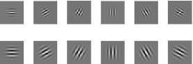
Gabor filters are parameterized functions useful for analyzing textured patterns. They efficiently represent different image regions since they scale, rotation and displacement invariant. A family of self similar Gabor wavelets closely models the simple cells of visual cortex making it a suitable choice for our application. Our experimental setup creates a Gabor filter bank for 4 scales and 6 orientations (window size 39x39) resulting in total

24 filters. Fig. 1 shows the magnitudes of Gabor filters. Fig. 2 shows the real parts of Gabor filters.

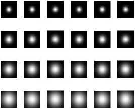
Fig.1. Magnitudes of Gabor Filters

ввивав

§ а И ПП ^ §

Fig.2. Real parts of Gabor Filters

For each scale and orientation, mean and standard deviation of magnitudes of transformed coefficients are calculated resulting in forty-eight dimensional feature vector. Figure 3 and Figure 4 show how an exemplar image is filtered using Gabor filter bank.

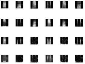
Fig.3. Magnitudes of Gabor Filtered Image

■■■■■■ ■■■■■■ й В ■ В ■ ■ ■ ■■■■■

Fig.4. Real parts of Gabor Filtered Image

Daubechies Wavelets

Wavelet Transform decomposes the image into a series of high pass and low pass bands and extracts directional details that capture horizontal (cH), vertical (cV) and the diagonal (cD) activity. Since lower spatial frequencies of an image are more significant for the image’s characteristics than higher spatial frequencies, further filtering of the approximation is useful. We use DB4 wavelets with three level decomposition (as shown in Fig. 5) similar to the approach used by authors in [3, 4].

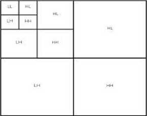
Fig.5. Daubechies three level decomposition

At each level of decomposition for HL, LH and HH sub-bands we calculate energy, mean and standard deviation resulting in a twenty-seven dimensional feature vector. Fig. 6 shows decomposition of an image using DB4 three-level decomposition. Fig. 7 shows the DB4 reconstructed image.

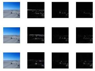
Fig.6. DB4 Three Level Decomposition of example image

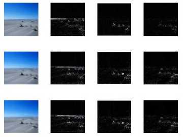
Fig.7. Reconstructed example image

Edges

In scene applications edges are dominant features. For example sky scrapers will have more vertical edges whereas mountain peaks will have prominent diagonal edges. To extract edge features we have used Edge Direction Histogram.

Edge Direction Histogram

The basic idea of Edge Direction Histogram is to build a histogram with the directions of the gradients of the edges (borders or contours). For scene images we are interested in the detection of the directions (angles) in which different edges occur. Edge Direction Histogram is used to describe the distribution of the edge points in each direction and is calculated by counting the number of the pixels in each user-defined direction. In [5] edge orientation along with other features has been used for indoor – outdoor scene classification based on neural network learning. In this paper edges are first detected using canny edge detector and edge pixels are counted in five directions vertical, horizontal, two diagonals and non-directional (which do not belong to any other category) resulting in a five dimensional feature vector. Table 1 summarizes the feature set used in our experiments.

Table 1. Feature set used in our approach

Feature	Description	Dimension
Color Moments(CM) (Z-score normalized)	Low     order moments mean, standard deviation   and skewness    in HSV space.	9
Color  Coherence Vector(CCV) (Normalized    by number of image pixels)	Two 27 bin histograms for coherent and non coherent regions	54
Color Correlogram (CC) (Implicitly in the form of probability)	Autocorrelogram at unit distance	64
GLCM   (Z-score normalized)	Six statistical features are calculated for each offsetangle pair	24
Daubechies Wavelets(DB4) (Z-score normalized)	Energy,  mean and    standard deviation     of coefficients obtained using three       level decomposition	27
Gabor    (Z-score normalized)	Mean, standard deviation of image filtered using 24 filters	48
Edge orientation/directio n histogram (normalized by number of edge pixels)	Count of edge pixels in 5 directions	5

• B.    Dataset used

  We have used the Oliva-Torralba dataset (OT) [16] which is a subset of the Corel database. The dataset description is given in Table 2. Experiment 1uses 1472 images from natural scene category (OT4 dataset). Examples are shown in Figures 8a-8p. Experiment 2 uses all 2688 images from eight categories (OT8 dataset).

Table 2. Category wise details of dataset used

Broad category	Internal category	Number of images
Natural	Coast	360
	Forest	328
	Mountain	374
	Open Country	410
Urban	Tall Building	356
	Street	292
	Inside City	308
	Highway	260
Total		2688 images

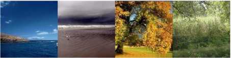
(a) Coast       (b) Coast

(c) Forest        (d) Forest

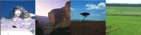
(e) Mountain (f) Mountain     (g) Open        (h) Open

Country        Country

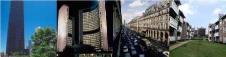
(i) Tall            (j) Tall           (k) Street        (l) Street

Building        Building

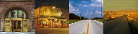
(m)Inside City (n)Inside City (o) Highway (p) Highway

Fig.8a-8p. Example images from each category.

• C.    Feature Fusion

Since no single feature can fully characterize an image we use feature fusion method with color, texture and edge features in this paper. Our system uses early fusion of feature vectors. Table 3 lists the fused feature combinations which have been evaluated for the two datasets in our experiments.

Table 3. Feature combinations generated after fusion

Fused Feature Set	Feature Vector Dimension
CM-Gabor-EDH	62
CM-GLCM-EDH	38
CM-DB-EDH	41
CCV-Gabor-EDH	107
CCV-GLCM-EDH	83
CCV-DB-EDH	86
CC-Gabor-EDH	117
CC-GLCM-EDH	93
CC-DB-EDH	96

CM is Color Moments, GLCM is Gray Level Co-occurrence Matrix, DB is Daubechies Wavelets, CCV is Color Coherence Vector, CC is Color Correlogram and EDH is Edge Direction Histogram.

• D.    Classifier Design

In this paper two discriminative models SVM and Artificial Neural Networks have been evaluated for scene classification.

SVM Classifier

Many authors have used SVM for scene classification. In [30] Gaussian kernel in an RBF-style classifier has been used. We have chosen SVM classifier because it is robust and effective even when less number of training samples is provided. This paper uses LIBSVM-3.20 package, dedicated for Matlab and have implemented One-Versus-All (OVA) technique for multi-class classification because it is faster, simpler and a complete approach. SVMs are parameterized by kernel function, box constraint constant C and a third constant depending on the type of kernel function used. The box constraint parameter C is the penalty parameter which controls the tradeoff between margin maximization and error minimization [25]. We have used Radial Basis Function (RBF) as kernel function therefore our SVM uses rbf_sigma as a parameter. For SVM tuning the training and test data has been normalized. Ten fold cross validation has been performed for automatic selection of C and γ values. The best parameters are used to train SVM using whole training set.

Artificial Neural Networks

Neural networks belong to a family of statistical learning models inspired by biological neurons and have been used by authors for various classification problems.In [3] authors have used probabilistic neural network for classification of scenes into indoor/outdoor category. In [4] two neural classifiers: back propagation neural network and resilient back propagation neural network have been used on varying number of feature vectors corresponding to scene images tested on scene classification MIT database.

We have chosen neural networks due to their self-adaptive ability. We have used a two layer neural network. The hidden layer size is 10. The training function used is ‘trainscg’ with learning rate set to 0.00001 and maximum number of epochs set to 5000.

• V.    Experimental Results

  The goal of our experiments is to classify an unknown image as one of the learned scene classes. We perform two sets of experiments on an Intel Core i3 processor with 4GB RAM using MATLAB 2012a to analyze the different aspects of our model and learning approach. Two classifiers ANN and SVM have been implemented using nine fused feature combinations on OT4 and OT8 datasets. Tables 4 and 5 present the results of scene classification of OT4 dataset and Tables 6 and 7 present

the results of scene classification of OT8 dataset by ANN and SVM respectively.

Table 4. Performance of OT4 dataset by ANN (Results obtained by cross validation)

Fused Feature Set	Fold Number					Peak Accuracy
	1	2	3	4	5
CM-Gabor-EDH	91.8	91.8	91.5	91.5	91.2	91.8
CM-GLCM-EDH	82.3	82.3	82	81.6	81.3	82.3
CM-DB-EDH	83.3	83.3	83	83	82.7	83.3
CCV-Gabor-EDH	89.1	88.8	88.4	87.8	87.4	89.1
CCV-GLCM-EDH	82.3	82	81.6	81.3	81	82.3
CCV-DB-EDH	76.2	75.2	74.5	74.1	73.5	76.2
CC-Gabor-EDH	74.1	71.7	71.1	70.7	70.1	74.1
CC-GLCM-EDH	71.8	69.4	69	66.7	66.5	71.8
CC-DB-EDH	74.8	73.8	73.5	73.1	72.8	74.8

Table 5. Performance of OT4 dataset by SVM (Results obtained by cross validation)

Fused Feature Set	C	Γ	Classification Accuracy
CM-Gabor-EDH	3.668	.016129	92.5
CM-GLCM-EDH	663.9819	.0012683	83
CM-DB-EDH	5.6569	.02439	83.7
CCV-Gabor-EDH	663.9819	.0010713	87
CCV-GLCM-EDH	534.6682	.001381	82.3
CCV-DB-EDH	279.17	.0020555	81.6
CC-Gabor-EDH	20.7494	.005422	86
CC-GLCM-EDH	20.7494	.0069723	77.5
CC-DB-EDH	76.1093	.0022868	79.2

Table 6. Performance of OT8 dataset by ANN (Results obtained by cross validation)

Classification accuracy of OT8 Dataset evaluation by ANN						Peak Perform ance
Fused Feature Set	Fold 1	Fold 2	Fold 3	Fold 4	Fold 5
CM-Gabor-EDH	85.1	84.5	84.2	84.2	84	85.1
CM-GLCM-EDH	81.6	80.4	80.3	79.9	79.7	81.6
CM-DB-EDH	78	77.3	77.1	76.9	76.5	78
CCV-Gabor-EDH	81.2	80.6	80.1	79.9	79.7	81.2
CCV-GLCM-EDH	76.9	76.2	75.2	74.7	74.3	76.9
CCV-DB-EDH	73.1	72.9	72.5	72	71.7	73.1
CC-Gabor-EDH	72.8	71.9	71.7	71.3	70	72.8
CC-GLCM-EDH	62.6	61.6	61.1	58.8	55.7	62.6
CC-DB-EDH	66.3	63.5	63.3	61.8	61.6	66.3

Table 7. Performance of OT8 dataset by SVM (Results obtained by cross validation)

Fused Feature Set	C	γ	Classification Accuracy
CM-Gabor-EDH	20.7494	.0043972	86.4
CM-GLCM-EDH	663.9819	.0018128	81.4
CM-DB-EDH	430.539	.0007622	78.4
CCV-Gabor-EDH	181.0193	.0020517	84.7
CCV-GLCM-EDH	430.539	.0050656	77.4
CCV-DB-EDH	663.9819	.00086425	76.5
CC-Gabor-EDH	5.6569	.020328	81
CC-GLCM-EDH	76.1093	.0045209	70
CC-DB-EDH	181.0193	.00077422	69.4

Table 8 presents the comparative results of classification using ANN and SVM.

Fig.11. Confusion Matrix of classification of OT8 dataset by NN

Table 8. Comparative Results of ANN and SVM

OT4 Dataset		OT8 Dataset
ANN	91.8	ANN	85.1
SVM	92.5	SVM	86.4

Confusion Matrix

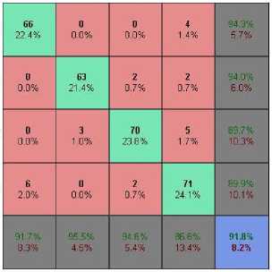
Figures 9 -12 show the confusion matrix for best performances reported by SVM and ANN over OT4 and OT8 dataset. Classes shown as 1,2,3,4,5,6,7,8 represent Coast, Forest, Mountain, Open Country, Tall Building, Street, Inside City, Highway.

Confusion Matrix

2          3

Target Class

50 10.8%	0 0.0%	1 0.2%	5 0.9%	0 0.0%	0 0.0%	0 0.0%	2 0.4%	67.9% 12.1%
0	61	0	2	0	0	0	0	96.8%
0.0%	11.4%	0.0%	0.4%	0.0%	0.0%	0.0%	0.0%	3.2%
1	2	69	2	4	0	0	0	88 5%
0 2%	0 4%	12 8%	0 4%	0 7%	0 0%	0 0%	0 0%	11 5%
8	3	4	72	0	0	3	2
1.5%	0.6%	0.7%	13.4%	0.0%	0.0%	0.6%	0.4%	21.7*1
0	0	0	0	60	0	3	1	93 8%
0.0%	0.0%	0.0%	0.0%	11.2%	0.0%	0.6%	0.2%	6.3%
0	0	n	1	2	54	7	2	81 8%
0.0%	0.0%	0.0%	0.2%	0.4%	10.1%	1.3%	0.4%	18.2%
и	0	0	и	5	4	4/	2	81.0%
0.0%	0.0%	0.0%	0.0%	0.9%	0.7%	0.8%	0.4%	19.0%
5	0	0	1	0	0	1	43	86.0%
0.9%	0.0%	0.0%	0.2%	0.0%	0.0%	0 2%	8.0%	14.0%
80.6%	92.4%	93 2%	86.7%	84 6%	93 1 %	77 0%	82 7%	86.4%
19.4%	7.6%	6.0%	13.3%	15.5%	6.9%	23.0%	17.3%	13.6%

1      2     3     4      5     6     7     8

Target Class

Fig.12. Confusion Matrix of classification of OT8 dataset by SVM.

Fig.9. Confusion Matrix of classification of OT4 dataset by NN

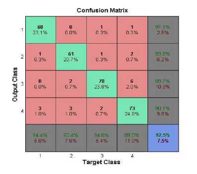
Fig.10. Confusion Matrix of classification of OT4 dataset by SVM

Table 9. Predictive accuracy on OT8 Dataset

Category	SVM			NN
	Sensit ivity	Speci ficity	F-score	Sensiti vity	Specif icity	F-score
Coast	.8056	.9828	.8406	.8333	.9871	.8696
Forest	.9242	.9958	.9457	.9091	.9894	.9160
Mountain	.9324	.9806	.9079	.9459	.9654	.8750
Open Country	.8675	.9559	.8229	.8554	.9604	.8256
Tall Building	.8450	.9914	.8889	.7606	.9807	.8060
Street	.9310	.9749	.8710	.8793	.9812	.8644
Inside City	.7705	.9769	.7899	.8033	.9748	.8033
Highway	.8269	.9856	.8431	.8077	.9897	.8485

Confusion Matrix

1162%	0.0%	0.0%	0.4%	0.0%	0.0%	0.0%	0.7%	90.9%
0.2%	11.2%	0.2%	0.4%	0.0%	0.0%	0.2%	0 0%	7 7%
0.2%	3 0.6%	13.0%	11%	11%	0.0%	0.0%	0 0%	16.6%
7 1.3%	3 0.6%	2 0.4%	71 13 2%	0.0%	0.0%	1 0.2%	5 0.9%	79 8% 20 2%
0 0.0%	0 0.0%	1 0.2%	0 0.0%	54 10.1%	3 0.6%	5	0 0.0%	85.7% 14.3%
0	0	0	0	3	51	0.9%	1	15.0%
0.0%	0.0%	0.0%	0.0%	1.5%	0.7%	49	0.0%	К
3 0.6%	0 0.0%	fl 0.0%	2 0.4%	0 0.0%	0 0.0%	0 0.0%	42 7.6%	89.4% 10 6%
16 7%	90 9% 9,1%	94 6% 54%	85 5%	76.1% 23.9%	67 9% 121%	80.3% 19,7%	80.8% 19.2%	B5.1%

1      2      3     4      5      6     7      8

Target Class

Other than classification accuracy we also report sensitivity (fraction of positive patterns that are correctly classified), specificity (fraction of negative patterns that are correctly classified), f-measure (harmonic mean of precision and recall values) and kappa statistic (a measure of agreement between the machine learning classifier classifications and ground truth labels). Table 9, 10 show the predictive accuracy measures of classification by SVM and NN on OT8 and OT4 dataset respectively.

Table 10. Predictive accuracy on OT4 Dataset

Category	SVM			NN
	Sens itivit y	Specifi city	F-score	Sensiti vity	Specific ity	F-score
Coast	.944 4	.9910	.9577	.9167	.9820	.9296
Forest	.924 2	.9825	.9313	.9545	.9825	.9474
Mountain	.945 9	.9636	.9211	.9459	.9636	.9211
Open Country	.890 2	.9623	.8957	.8659	.9623	.8820

Table 11 reports the average accuracy measures.

Table 11. Average Performance Measures

Predictive measure	Dataset OT4		Dataset OT8
	SVM	NN	SVM	NN
Sensitivity	.9252	.9184	.8641	.8510
Specificity	.9751	.9728	.9806	.9787
F-score	.9252	.9184	.8641	.8510
Kappa statistic	.899	.8864	.844	.829

• VI.    Analysis of Results

We have performed our experiments on two types of datasets- One which contains only natural scenes and the other which contains both natural as well as man-made structures. Many cases are very easily separable due to the different color, textural and/or structural composition. However the dataset used also contains overlapping classes. To solve this problem our aim was to find feature extraction methods that suited the domain and separated the classes better. State of the art feature extraction methods (color, texture and edge directionality features) and classification methods (Artificial Neural Networks and Support Vector Machine) were tested and the best of these were selected to be used in final scene classification system. We have used supervised learning algorithms for classification because they are able to learn with few images to facilitate the task of scene categorization. In order to evaluate the goodness of the implemented system a comparison between the results of the classifications and use of different feature sets has been presented in Section V. This section presents an analysis of the obtained results.

• A.    Classifier Evaluation

Specifically, to know the performance of the system a confusion matrix is computed. This is to check if the system is confusing two classes that is mislabeling an image of one class to another class. A confusion matrix shows the number of correct and incorrect predictions made by the classification model compared to the actual outcomes (target value) in the data. The overall performance rates are measured by the average value of the diagonal entries of the confusion matrix since they represent the number of correctly classified images. The off diagonal elements give us the false positives and the false negatives and thus represent the classification errors.

SVM performs better in both OT4 as well as OT8 datasets than Neural Networks in terms of classification accuracy. SVM gives peak classification accuracy of 92.5% for natural images in OT4 dataset and 86.4% for natural and urban images in OT8 dataset. The sensitivity and specificity values for SVM classifier for OT4 dataset as shown in Table 11 are .9252 and .9751 respectively. For OT8 dataset these values are .8641 and .9806 respectively. These high values indicate that the classifier is good at detecting the positives. At the same time SVM is capable of avoiding false alarms. Even though SVM performs better than NN in both datasets yet the performance can be greatly improved for OT8 dataset. We have also evaluated the kappa statistic to establish agreement between the expert and the classifier. In case of OT4 and OT8 dataset the kappa statistic value is .899 and .844 respectively. These high values indicate that the assignment of an image to a class is not random; rather the system has been well trained to classify the images. This shows the excellent classification ability of the classifier.

• B.    Study of Misclassifications

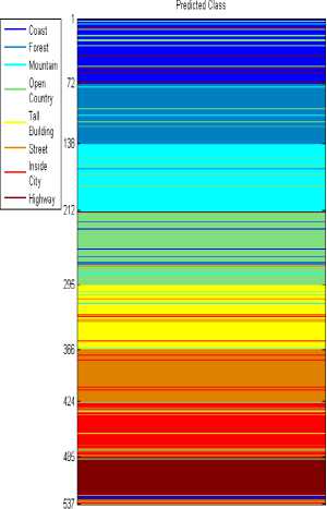
Figure 13 and 14 show the actual and predicted class (test images) for OT4 and OT8 datasets by SVM.

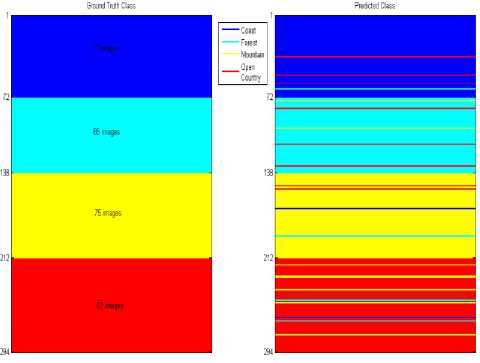
Fig.13. Actual versus predicted class OT4 dataset

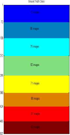
Fig.14. Actual versus predicted class OT8 dataset

In Figure 13 we can see that there are 72 test images of Coast class, 65 of Forest class, 75 of Mountain class and 82 of Open Country class.

Coast images are often misclassified as open country images (3/72). This is shown as red lines in the blue patch. There seems to be confusion between images from mountain and open country categories. 2/74 mountain images are classified as open country. It is also observed that open country images are misclassified as mountain images (6/82). This is shown as shown as yellow lines in the red patch.

The classifier is capable of distinguishing between coast and forest images. Only one coast images is classified as forest image (1/72). None of the forest images are classified as coast images. Forest images are misclassified as mountains and open country images may be due to occurrence of foliage making them semantically similar thus causing ambiguity.

As shown in Figure 14 Tall building images are classified into Inside City category (5/71). There also seems to be ambiguity between Street and Inside City images. 4/58 times street images are put into Inside City category and 7/61 times Inside City images are classified as street images. This may be due to the less expansiveness of both kinds of images. Highway images are misclassified as Street and Inside City images.

• B.    Feature Evaluation

The tests show that with the combination of best features, the accuracy of SVM is 92.5% and 86.4% for OT4 and OT8 dataset respectively.

In the case of different color features Color Moments produced good classification results than Color Coherence Vector and Auto Correlogram. Thus, among color features Color Moments are more discriminative. Among texture features the features extracted using Gabor filters are more discriminative than GLCM and Daubechies wavelets. The Edge direction histogram is discriminative as it identifies edges appropriately to distinguish between natural and urban images and also among categories of natural images.

• C.    Performance Benefits of Selected Features

Our system has achieved highest classification results with the combination of Color moments (color features), Gabor filters (texture features) and Edge histogram (edge distribution) since these features were compact within a category and distinct for different categories. We have performed feature level fusion which is advantageous because it utilizes the correlation between multiple features at an early stage which helps in better classification rate.

Lower order color moments are invariant to illumination and viewpoint and have efficiently interpreted the distribution of color in scene images. 2-D Gabor filters allow the study of the spatial distribution of texture. In the problem of scene classification Gabor filters have enabled the detection of gradual changes of texture and texture variations since the frequency and orientation representations of Gabor filters are similar to those of the human visual system. To capture rough global shape structure in an image edge direction histogram has been used which efficiently defines the distribution of direction of each edge pixel.

The comparative performance of various scene classification systems found in literature is given in Table 12. We have reported best classifier and feature combination of our work in this table.

Table 12. Performance Comparison

Author	Approach	Features	Classes	Result
Our Proposed Method	SVM	Color Moments , Gabor features, Edge Direction Histogram	4	92.5
Gupta et.al [14]	FeedForward Neural Network	Color Moments (RGB), Daubechies wavelets	3	82.66
Grossberg and Huang[22]	Neural system	Surface color statistics, Three principal textures	4	91.85
Han and Liu [7]	Kernel PC based prototype presentatio n	Color opponent features, Spatial layout of Gabor features	4	91.3
Oliva and Torralba [15]	K-NN classifier	Naturalness, Openness, Roughness, Ruggedness, Expansion	4	89

• VII. Advantages of Proposed Approach

This paper addresses the problem of scene classification without the need of segmentation and the processing of individual objects or regions thereby representing a scene image using a set of global image properties. The main aim of this work is to classify scenes using global low-level features.

Highlights

Though different authors have attempted to derive global semantics from low-level features but the uniqueness of the approaches proposed in this paper are:

• 1)    We propose a global-feature-based-system to derive semantics from images. The training and test images are not divided into sub-blocks / subimages which saves computation time and complexity and also results in reduced feature set derived holistically.

• 2)    The proposed work does not rely on object recognition or object occurrences and their mutual relations as inaccurate segmentation can decrease categorization accuracy.

• 3)    No involvement of human subjects like other approaches [15] to rank training images based on different properties (such as ruggedness, expansiveness and roughness etc.).

• 4)    No requirement of classifying a large number of local patches [6] into semantic concepts (such as water, foliage, sky etc.) in order to train concept classifiers.

• 5)    No semantic annotations or keywords of training images are required in the proposed system.

• VIII. Conclusions and Future Directions

The high classification accuracy achieved for natural images as well mixed images from natural and urban categories reveals that discriminative properties can be inferred from low-level image features. Low-level strategies for semantic scene classification have two clear advantages: their simplicity and their low computational cost. The classification of eight scene classes is complex since many images in different scene categories are very similar and ambiguous taking their semantic content into account. The class boundaries are not clear and in many cases the classes were not easily separable.

The major contribution of the work presented in this paper is successful semantic scene classification by the best combination of low-level features. After exhaustive experimentation we have found that the combination of holistic features (Color Moments-Gabor features-Edge direction histogram descriptors) proves to be the best in both SVM and Neural Network classifier. Increasingly, the research community has been pursuing the clear alternative of semantic features and we can derive midlevel features from the best combination of low-level features found in this work in order to reduce the “semantic gap”. Intuitively we would also like to evaluate our method on other benchmarked datasets as well to check the effectiveness of the best features found so far. Our further research would be in two promising directions: Firstly to group a given collection of scenes into meaningful clusters according to the image content without a priori knowledge in an unsupervised manner allowing the system to extract meaningful patterns and association rules from clusters and secondly learning symbolic and / or semantic features from scenes using low-level features which should help bridge the semantic gap.