Image compression using discrete orthogonal transforms with the «Noise-like» basis functions

Discrete orthogonal transforms (DOT)

N - 1

x ( m ) = ^ x ( n ) h_m ( n ), m = 0,1,..., N - 1 n = 1

are widely used in the fields of information coding, information transmission and discrete signals processing. Here x ( n ) is the N-periodic input sequence, { h m ( n ) } N - 0 are the basis functions orthogonal for some scalar (or Hermitian) product.

• < h u , h v >= 5 uv

In the real world channels the noise distorts the transmitted signals, especially those with the low numerical values. If the channel characteristics are such that some samples of the transmitted information can be irretrievably lost or strongly distorted regardless of their values then standard DOTs (Fourier, Hartley etc.) can hardly be used for information coding. The standard DOT properties depend on the correlation properties of the processed signal. Therefore the loss of some high amplitude components (for example Fourier components) during the videoinformation transmission results in a strong noise in the restored image. This noise has periodic structure for which the human vision is very sensitive.

Another decision in this case is to code the information with the DOTs having such basis functions h_m ( n ) for which the spectral components { x ( m ) } are «ener-getically equal».

The notion of discrete M-transforms with the noiselike discrete functions is introduced in [1]. The applications of such transforms for one - and two - dimensional information coding are considered in [2]-[4].

Such transforms do not lead to energy concentration in a few spectral coefficients do not lower the redundancy attributed to the statistical relations between the elements of the signal to be transformed and efficiently remove insignificant information.

Particularly in the process of compressiondecompression of videoinformation after the inverse transformation was applied, the noise affecting the image is less notable for the human vision than in case of Walsh transforms.

The basis functions of such transforms are based on the m-sequences (recurrent sequences of the finite field elements with the maximum periods) The sequences of this kind are widely used for the pseudorandom numbers generation, cryptography etc [3]-[4].

The M-transforms with the basis functions taking two different values with the (nearly) equal frequencies are considered in the publications mentioned above. In our article we consider the generalized M-transforms with the basis functions taking p different values. The two-dimensional versions of the proposed structures are also discussed.

• 2.    Generalized one-dimensional M-transforms

Let F p be the finite p -element field. Let ф ( n ) be the r -order recurrent sequence

ф (n ) = a 1 ф (n - 1) + ... + а _г ф (n - r ), a j e F p      (1)

with nontrivial initial values ( ф (0),..., ф ( r - 1)).

Definition 1 Let N be the period of sequence (1). If

N = p^r - 1 then sequence (1) is called the m-sequence.

Using the slight modification of the corresponding proof [1] the following statement can be proven:

Proposition 1 Let p be prime, N = p^r - 1. Let the numbers A 0 ,..., A p । satisfy the following relation

, Ap - 1 ^- A 0

A k = ^k -------"---+ A 0 , ^{( k} = 0,..., p ^- 1)

p ^{- 1}

Let the functions h_m ( n ) be determined by the following relations

• 1    h o( n ) = A k          if ф ( n ) = k ;

• [    h_m ( n ) = h o( m + n ) if ф ( n ) * k .

Then there exists the efficiently calculated constants

A ₀ and A k such that the functions { h_m ( n ) } N - 0 form the orthonormal set

N - 1

< ^h u , ^h v >= ^, h u h v = 5 uv n = 0

Proof. Let us introduce the following notation

A p - 1 ^- A 0

C =-----------, hr (n) = h o( n + т), A о = A p -1

H k ( ⁿ ) =

• 1, if ф ( n ) = k ;

• 0, if ф ( n ) * k .

Then p-1

h T = Y ( A + kC ) H k ( n + т )                  (2)

k = 0

Let us take A q and A p - 1 that the orthogonality condition for the set { h m ( n ) } is held in the form

N - 1

< h _T , h v >= N ^{- 1} £ h _T ( n ) h v ( n ) = S „         (3)

n = 0

Since the functions h _T are obtained from each other by the cyclic shifts then the sum (3) depends only on ( t - v ). Therefore we can consider only the case of v = 0.

Using (2) and (3) for т = 0 we get

N - 1 N - 1

N = £ ( £ ( a + Ck ) H k ( n )) ²               (4)

n = 0 k = 0

Since Hi (n) H j (n) = Sij then using (4) we obtain p -1 N -1               p -1 N -1

N = A ² £ £ H i ( n ) + 2 AC £ i £ H i ( n ) i = 0 n = 0                  i = 0 n = 0

p - 1 N - 1

+ C2 £ i2 £ Hi (n) = i = 0

p -1

= A2N + 2AC £ ipr-1 + C2 £ i2pr-1 = i=1

= A ² ( p^r - 1) + ACp^r ( p - 1) +

+ c 2 pr (p - 1)2p-1(5)

Let t * 0. Then we have p -1 p -1

0 =££ (A + Ci)(A + Cj ) Sij (t )(6)

i = 0 j = 0

Here

N - 1

Sij (t ) =£ Hi (n)Hj (n + т).(7)

n = 0

The calculation of Sij is the most difficult part of this poof. Using the standard method from number theory we can bring (7) to the trigonometric sum of the special kind.

Let Л be the nontrivial character of a field F_p r = F q additive group. Then

q

- 1

£ ло ) ^{a e} F_q

1, if в = 0;

0, if в * 0.

(see [4]).

The following condition holds for m- sequences

N - 1

£ ^{л (} ф ⁽ n )) = - i.

n = 0

Thus

N - 1

S ij ^{( t} ) = q ^{- 2} £ ( £ ^{л ( а} ( ф ⁽ n ) ^- i )))

n = 1 ae F„

q

^{x (} £ ^{Л ( в (} ф ( n + т ) ^- j ))) = ве F_q

= q ^{- 2}     £ Л   ( - a - e i ) ^x

^{( a} , ^{в ) e} F q ^x F q

N - 1

x £ Л ( а^ ( n ) + рф ( n + т ))

n = 0

Since for ( a , в ) * (0,0) e F_q x F_q the functions

Ф ^р ( n ) = «ф ( n ) + вф ( n + т )

are the m-sequences then

S ij ( t ) = q ^{- 2} N - q "²        £ Л ( -a i -в)    (8)

( a , в ) e F q x F q \{ O }

Since

A             f q ², if i = j = 0

£     Л ( -a i ) Л ( - Pi ) = 5

(a,в)eFqxFq                       10 , else then

S ij ( t ) = q -2 N - q "²      £ Л ( - a ) Л ( - р )

^{( a} , ^{в ) e F} q ^{x F} q

+ q ² £ ^{л (} - o i ') + q ² £ ^{л ( - p ) -} q ² = ^{a e F} q              ^{ве F} q

• ' q "2 N - q -2,              if i , j * 0

• = q ² N + q - q ² , if i = 0, j * 0

or i * 0, j = 0

• . q ^{- 2} N - 1 + 2 q ^{- 1} - q ^{- 2} ,   if i = j = 0

• 3.    Two-dimensional GM-transforms

Substituting S ij ( t ) in (6) we get an explicit relation between A and C . This relation together with (5) brings the system of equations for determining A and C and therefore A ₀ and A_p - 1 .

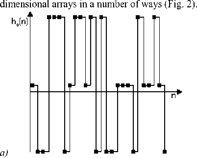
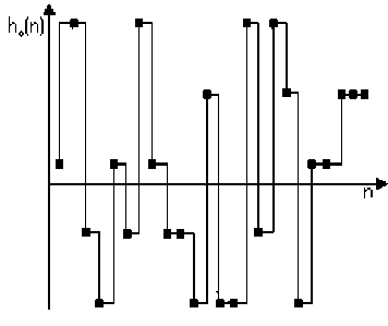
The examples of the basis function h ₀ ( n ) for different p and N are shown on the fig. 1.

Definition 2 The transform (1) with the basis functions { h m ( n ) } defined in Proposition 1 is called the generalized M-transform (GM-transform).

The one dimensional M-transforms introduced in the previous section can be used for two-dimensional digital arrays (images) coding after the standard digital image processing methods were applied.

• (a) The N×N pixel images can be represented by one-

  
  
  
  
  
  

  x ( m i , m 2 ) =

  
  

N - 1 N - 1

= ∑ ∑ x ( n ₁, n ₂) h_{m 1} ( n ₁) h_{m 2} ( n ₂) n ₁ = 0 n ₂ = 0

In case (a) the two- dimensional N×N-points GM-transform calculation is reduced to the calculation of one- dimensional N²-points GM-transform. In case (b) the two- dimensional N×N-points GM-transform calculation is reduced to the calculation of N one - dimensional

N-points GM-transforms. This calculation is done using the standard “row-column” (cascade) scheme:

b)

N - 1 N - 1

^{x (} m 1 , m 2 ) = ∑ ( ∑ x ( n ₁, n ₂) h _{m 1} ( n ₁)) h _{m 2} ( n ₂) n ₁ = 0 n ₂ = 0

Fig. 1. Function h ₀ ( n ) for (a) N=26, p=3, r=3, (b) N=24, p=5, r=2

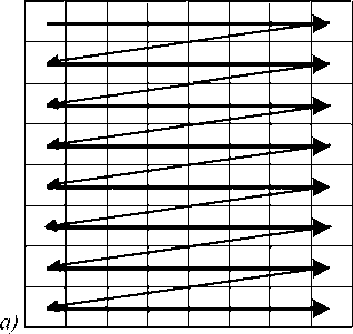
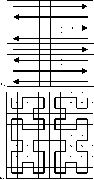
Fig. 2. Different ways of representing two-dimensional N×N array as a one-dimensional N2 – element array.

(b) We can introduce the separable two-dimensional GM-transform by the following relation.

• 4.    Fast algorithms for GM-transforms

The main property of GM-transforms is the existence of fast algorithms of their calculation.

Let us show that transforms (1) and (9) can be represented in a form of one- and two-dimensional convolution respectively.

Let η =- n , η ₁ = - n ₁, η ₂ = n ₂.

The signal x ( n ) and the functions h _m ( n ) are N-periodic. Thus considering the introduced notation expressions (1) and (9) can be transformed into

N - 1

x ( m ) = ^ x ( n ) h ₀( m - n ) = ( x * h )( m )          (10)

η = 1

x ( m i , m 2 ) =

N - 1 N - 1                                     ₍₁₁₎

= ∑∑ x ( n ₁, n ₂) h ₀( m ₁ - η ₁) h ₀ ( m ₂ - η ₂) η ₁ = 0 η ₂ = 0

Array (10) can be calculated in a standard way using the discrete Fourier transform (DFT).

DFT

Inverse DFT

J(X)----------- ► *^hoXm)

DFT     / hM---->H^nT)/

Fig. 3.

The drawback of this scheme is that N = p ^r - 1can hardly be factored as

N = p ₁ ^{α 1} ⋅ ... ⋅ p ^α t ^j                                     (12)

The numbers p ₁ ,..., p_t in (12) are primes.

The DFT calculation for N = p ₁ ^{α 1} ⋅ ... ⋅ p ^α _t ^j can be done using Good-Thomas decomposition [6]. According to it we have to calculate p ^α _j ^j -point DFT ( j = 1...... t ). There exists efficient FA for all p j .

Another decision in this case is to calculate (10) and (11) using polynomial transform method [5].

The detailed discussion concerning the fast algorithms for calculation of (10) and (11) will be given on presentation.

• 5.    Experimental results

Figures 4b-4d illustrate the reconstructed images after 70 of 256×256 spectral components have been replaced by zeroes for Hartley transform (b), Hadamard transform (c) and GM-transform (d). The original image is depicted on Figure 4a. The «lost» transforms were chosen in a random way.

The more detailed discussion concerning the restoration quality will be given on presentation.

b)

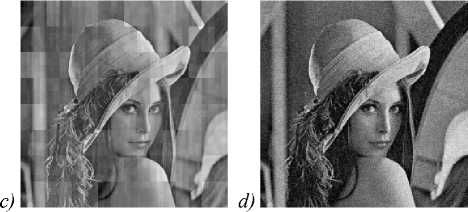
Figure 4. (a) Original image, (b) Hartley transform, (c) Hadamard transform, (d). GM transform

• 6.    Conclusion

In authors’ opinion the capabilities of GM-transforms are not limited to the examples given in the article. It is clear that GM-transforms can be used for signal processing not only in the frequency field but also in the time field. Such problems arise when processing (in particular, when interpolating) non-uniform sampling signals [7]-[8].

Acknowledgement

This work was performed with financial support from the Russian Foundation of Fundamental Investigations (Grant 97-01-00900).