Image Retrieval Based on Color, Shape, and Texture for Ornamental Leaf with Medicinal Functionality Images

Published Online June 2014 in MECS DOI: 10.5815/ijigsp.2014.07.02

Human has a duty to preserve the nature. One of the examples is to preserve the existence of the plant. There is a necessity cycle between human and plant. Plant produces oxygen from photosynthesis process, and human provides carbon dioxide that vital for plant. Logically, human will experience problems when number of the plant is gradually reducing. This research uses leaf from ornamental plant as a plant that need to be preserved. Ornamental leaf because of its main function as ornament certainly has sale value. Maintaining the preservation of this plant will give many benefits in many aspects to the human itself.

Based on International Union for Conservation of Nature and Natural Resources, the number of identified plant species in the world which consist of Mosses (M), Ferns and Allies (FA), Gymnosperms, Flowering Plants (FP), Red and Green Algae (RGA) is about 307.674 species [1]. Fig. 1 shows the number details.

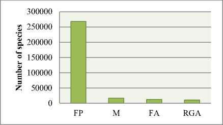
Fig 1: Column charts number of identified plant species

On the other side, the approximate number of unidentified species is 86.429 species. It consists of Flowering Plants with 83.400 species, Ferns and Allies with 3.000 species, Mosses with 29 species [2]. Considering the highest number possessed by Flowering Plants, identification of the plants, which include also ornamental plant, has become a challenge for us.

As recognition step of unidentified species, this research is focusing on ornamental leaf that functioned as medicinal leaf. However, only few people know about its function as a treatment of the disease. In Indonesia, this plant is also easy to find because mostly cultivates in front of the house. If its medicinal function and that easiness are taken into consideration, this plant should be an initial treatment or an option towards full chemicalbased medicines.

Identification of leaf image is possibly done through identification of some leaf features, i.e. color, shape, and texture. Previously, most of the researchers were using shape and texture feature to identify the leaf. In 2000, Wang et.al [3] proposed leaf image retrieval using shape features. Leaf shape characterized by centroid-contour distance curve and object eccentricity functions. The eccentricity is used for rank the leaves and its best ranked result is further re-rank again using the centroid-contour distance curve.

Followed by Park, Hwang, Nam [4] in 2007, they were employing curvature scale scope corner detection method to detect the leaf venation. Categorization of the selected points is managed by calculating the density of feature points. We also have been proposed this ornamental leaf identification through classification [5]. SVM acted as a classifier with features elements exactly same with this research. In previous research, we gained favorable average performance results.

Shape is a substantial part to describe image content, and shape of this ornamental leaf is very diverse. From texture feature, we can obtain one of the important information from leaf called leaf venation. Subsequently, color information is still considered as an additional feature, despite the dominant color of ornamental leaf is green. In HSV model, we can get information from color differences in respect to black, white, and lighting.

This paper is organized as follows. Explanation about ornamental leaf that used in this research is in section II. In section III, we explain the proposed method that consists of leaf features extraction, flowchart of this research, and Bayesian automatic weighting formula. Section IV describes about experiment and result. Conclusion and future work will be the end section of this paper.

Firstly, boils the leaf together with water and apply as drinks. Secondly, put the leaf to the skin surface [6].

Table 1: Medicinal function of ornamental leaf

Name	Medicinal function
Gardenia	Sprue, fever, constipation
Bay	Diarrhea, scabies and itching
Cananga	Asthma
Mangkokan	Mastitis, skin injury, hair loss
Cocor Bebek	Ulcer, diarrhea, gastritis
Vinca	Diabetes, fever, burn
Kestuba	Bruise, irregular menstrual
Jasmine	Fever, head ache, sore eyes

• II.    Ornamental leaf as medicinal leaf

Ornamental leaf on this research is not general ornamental leaf. This ornamental leaf has two general functionalities. First as an ornament in open space, and second as herbal medicine that used to cure some diseases.

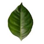
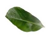
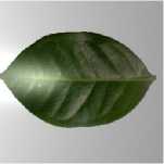
Image dataset of ornamental leaf on this research is obtained by direct acquisition using a digital camera. This dataset consists of tropical ornamental plants’ images that usually cultivate in front of the house. This dataset contains 8 classes with 15 images for each class. The classes are Gardenia ( gardenia augusta, merr ), Bay ( syzygium polyanthum ), Cananga ( canagium odoratum, lamk ), Mangkokan ( nothopanax scutellarium merr .), Cocor bebek ( kalanchoe pinnuta ), Vinca ( catharanthus roseus ), Kestuba ( euphorbia pulcherrima, willd ), Jasmine ( jasminum sambac [soland] ). These plants are not affected by the seasons, and it will be able to grow-up for one whole year. In order to avoid expensiveness of computation, size of the image is 256 x 256 pixels. Fig. 2 contains sample images from all classes.

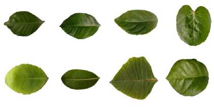
Fig 2: Sample Images from all class. From upper left to lower right: gardenia, bay, cananga, mangkokan, cocor bebek, vinca kestuba jasmine.

Table 1 shows specific medicinal function of corresponding ornamental leaf. In Indonesia, there are two mostly used serving ways of these ornamental leaves.

• III.    Proposed methods

• A.    HSV-based color histogram

The widely used color model called RGB only defines a color using a combination of primary color. Different with RGB, HSV color model defines color similarly to how the human eye tends to perceive color. HSV color model represented by a hexacone with center vertical axis is intensity [7]. Hue represents color type, and it consists of red at angle 0, green at 2π/3, blue 4π/3, and red again at 2π. Saturation is depth of color and measured as radial distance from the central axis to the outer surface.

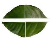
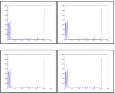
In this research, instead of engaging a global approach histogram, which one whole image is measured by one histogram, we propose to use local approach histograms, which one whole image is separated into 4 parts and measure its histograms. Because the color is limited to green, the numbers of hue and saturation bins are 4 and 3 bins, respectively. As an illustration, refer to Fig. 3.

(a)

(b)

(c)

Fig 3: Local approach color histogram. (a) original image, (b) sliced images, (c) histogram of each slice

7.    =

,   ⁼

n+1 λN

n+1 λN

N-lN-l

∑∑f(a, b)V ^∗,m (a, b) a=0 b=0

N-lN-l

∑∑f(a, b)Rn (ρab)e-imeab a=0 b=0

Where λN is normalization factor and 0≤ρab≤1. Transformed distance ρab and the phase θab at the pixel position (a,b) are showed with following equations:

√(2а-Ν+1) ² +(2b-Ν+1)     ⁽⁶⁾

ρ ab =

• B.    Zernike complex moments

The Zernike complex moments can be obtained utilizing these following steps:

• 1.  Computation of radial polynomials

• 2.  Computation of Zernike basis functions

• 3.    Computation of Zernike moments through projecting the image onto its basis functions

First step is computation of radial polynomial and represented by the following equation:

θab

=tan -1

Ν-1-2a

2а-Ν+1

The magnitude of Zernike moments from original image with rotated image will be equal.

This rotation-invariant ability become a reason to propose this method as shape feature extractor method. This research only used low-order of Zernike complex moments because of computation inexpensive and not sensitive to the noise [8,9]. The following table shows the proposed low-order Zernike complex moments:

(     )/

∑(-1)к()

k!(   -k)!(   -k)!ρ

n and m are representing the order and the repetition of azimuthal angle, respectively. The length of vector from original point to point ( x,y ) denoted by ρ.

From (1), complex two-dimensional Zernike basis functions are constructed by:

Vп , m(ρ,θ)=Rп (ρ) jme,    |ρ|≤1       (2)

The following orthogonality condition is satisfied by the complex Zernike polynomials:

г 2П г 1

^0   ^0

V ^∗ , m (ρ, θ)Vр , q(ρ, θ)ρԁρԁθ

π n+1

; n=p,m=q

; otherwise

Table 2: Low-order Zernike complex moments

Order n	Iteration m	Number of moments
3	1,3	2
4	0,2,4	3
5	1,3,5	3
6	0,2,4,6	4
7	1,3,5,7	4
8	0,2,4,6,8	5
9	1,3,5,7,9	5
10	0,2,4,6,8,10	6
Total moments  32

Sign * denotes complex conjugation. This orthogonality defines no redundancy inter-moments with different order and repetitions.

Here is the definition of the complex Zernike moments n+1  2" Г1                       (4)

ZП,m=ⁿ⁺_π ∫  ∫f(ρ,θ)V ^∗ ,m(ρ, θ)ρԁρԁθ    ^{( )}

^π Jo Jq

Image function, f(a, b), for digital images can be replaced by summation operation.

The discrete Zernike moments for image with size N x

N is defined as

• C.    Dyadic wavelet transform

The downsampling wavelet, which samples the scale and translation parameters, is often fails when deal with some assignments such as edge detection, features extraction, and image denoising [15]. Different with the downsampling wavelet, the dyadic wavelet samples only the scale parameter of a continuous wavelet transform, and does not samples the translation factor. In one side, it creates highly redundant signal representation, but the other side, since it has shift-invariance ability, this method is a convincing candidate as a texture feature extractor method.

Let L² (R) be the space of square integrable functions on real line R, and define the Fourier transform of the function ф E L²(R ) by

^(to) = J   ()f)e-^iMtdt

If there is exist A > 0 and В such that

Z OO

|^(2⁷w)|  

then 1(t) is called dyadic wavelet function. Dyadic wavelet transform of /(t) is defined using this ф (t) by

1   t-u

Wf (u,27) = J  /(t) —1(),

V2727

from (9), 1^(0) = 0 must be satisfied, i.e., J°1(t)dt = 0. In order to design the dyadic wavelet function, we need a scaling function (t) satisfying a two-scale relation

h(to)h.*(to) + д(ш)д(ш) =2, to E [-тт,тт], where * denotes complex conjugation. This condition called a reconstruction condition.

Under condition (15), we have aj+1[n] = ^ h[k]a7-[n + 27k]; ; = 0,1, ...,

к

d]+1 [n]=Zka[k]a7[n + 27k];; = 0,1 here a0[n] is given by a0[n] = JO/to^t - n)dt.

The (16) and (17) are dyadic decomposition formula for one-dimensional signals.

Texture feature elements from this method are represented by energy, mean, standard deviation, and coefficient of variation. We propose to extract those values from approximation, horizontal, vertical and diagonal sub-images. The following image shows the details:

ф(t) = ^ h[k]V2(2t - k).

A—>k

The scaling function ф (t) is usually normalized as /_” (t)d t = 1.

By (11), the Fourier transform of the scaling function resulting

#<«» = ХЮ'

where h denotes a discrete Fourier transform

Я(Ш) = ^h[k]e-^

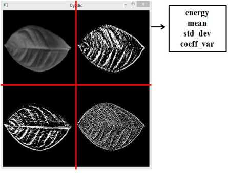
Fig 4: Texture feature elements represented dyadic wavelet transformation

Since <Я(0) = 1, we can apply (12) and (13) to obtain h(0) = V2. Using the scaling function and the wavelet filter 5 [k] , we define a dyadic function by 1(t) = 5ks[fc]V2/(2t-k).

The Fourier transform of 1(t),

#WX(>Q

will be needed later.

Let us denote the discrete Fourier transform of the filters h[k], h[k], h[k], and g[k], by h(h(to), Я(<у) and g(to) respectively. We suppose that these Fourier transforms satisfy the below condition

Because wavelet works in the frequency domain, energy is very useful as a feature extraction element. Energy values from several directions and different decomposition levels can possibly well-capture the leaf main information which called leaf venation. The other component is mean value, and it can be interpreted as central of tendency of the ornamental leaf data. When standard deviation or predictable dispersion increases in proportion to concentration, we have the other value as a solution called coefficient of variation. Through these comprehensive and fully-related values, we believe that we can gain satisfying results.

• D.    Flowchart

The following image is the flowchart of this research.

Leaf images

database

I

Segmentation

Features

Extraction

Query image

Right part of above equation can be modified with

P(C, S, T |Q) =P(Q|C, S, T) ×

P (C, S, T) P(Q)

Color: HSV

color hist

Shape: Zernike

Texture: Dyadic

moments

wavelet

Features

database

can be replaced with the constant α, as far as query Q is exist with the same probability. It’s simplified through following rule:

1,if аll feаtures exist in query Q    (20)

P(Q|C, S, T) = {0, otherwise

The (18) can be modified with

P(Ii|Q) =α[1-Р(C̅ |C) ×P(S̅|S) ×P(T̅|T)]      (21)

Calculation for each feature can be done separately, as an example for color feature

Similarity

Bayesian weighting measurement

Fig 5: Flowchart of this research

p ( ̅| c )=

( ^̅ ∧  )

~P ( C )

Aforementioned is a constant for images inside the database denoted by α, above equation can be rewritten as

P ( ̅| c )= a P ( ̅ ∧ C )

Based on the above flowchart, there are two inputs of this image retrieval system, ornamental leaf images database and a query image. The input’s features are extracted using three aforementioned methods, which are HSV-based color histogram to extract color information, Zernike complex moments as shape information extraction method, and texture information represented by elements from Dyadic wavelet transformation.

All of features extraction elements from every image in the database are stored in the database. Further step is the similarity calculation using Euclidian distance between images in the database and query image for color, shape, and texture features. Then, these distance values are weighted automatically utilizing the Bayesian automatic weighting formula to get single final representation distance. This formula adjusts the weights for all features and has a purpose to obtain maximum performance of this retrieval system. The sorted distance values as ranked result of this retrieval system.

E. Bayesian automatic weighting formula

Image I j with features color C , shape S , and texture T if given query Q will be exist with the probability

P(Ii|Q)=∑Р(Ii, C, S, T|Q)               ⁽¹⁸⁾

C,S,T

= ∑ Р(I, | C, S, T)

C,S,T

× P(C, S, T|Q)

As seen in (21), we can apply to the entire probability

P ( Ij | Q )= a [1- P (̅̅̅ | C )× P ( ̅ | S )      (24)

× p (̅̅̅ | T )]

p ( Ij | Q )= a [1-(1- P (̅̅̅ | C )) × (1      (25)

_- P ( ̅ | S ))×(1

^^^^^^^^^^^^™

^- p (̅̅̅ | T ))]

The above equation is the final equation for this Bayesian weighting formula.

F. Evaluation

Recall and precision values are the most common values in image retrieval area used for system effectiveness measurement. Recall value is the division between the number of relevant image retrieved and number of relevant images. The division between the number of relevant images retrieved and number of retrieved images is the definition of precision value. The proper system will have precision values decrease when the number of retrieved images is increased.

#relevаnt imаges retrieveԁ       (26)

eса        #relevаnt imаges

#relevаnt imаges retrieveԁ      (27)

Preсision =

#retrieveԁ imаges

For evaluation step, in order to attain smooth recallprecision graph, utilization of the interpolated precision

value is proposed. The precision values in this step are the average precision values from all images in one ornamental class. These precision values of various recall values will be interpolated to its maximum precision value. In this research, we have 8 classes with 15 images for each class. It means there are 15 sets of precision values to be averaged out, and 8 sets to be interpolated. The following equation describes the detail:

p ipl (r) = mаx p(r′)                (28)

r/>r where pipl is the interpolated precision value, and r is certain recall value, recall level r’ ≥ r.

• IV. Experiment and result

• A.    Leaf Image Datasets

  Leaf Image datasets of this research consist of original (no change at all), rotation, scaling, translation, perspective changed, and lighting changed. Inside the rotated dataset, there are images with dissimilar degrees of rotation start from 45⁰, 90⁰, 135⁰, 180⁰, 225⁰, 270⁰, and 315⁰. For scaled dataset, we have 30% and 60% downscaled images.

Then, for the translated dataset, we translated the images to many directions within the original image size. The further dataset is perspective changed dataset, which two different perspective changes applied into the images. The last is lighting changed dataset where dominant part of the image is affected by lighting source. Fig. 6 shows sample images of all datasets:

• B.    System performances using recall and precision values

Table 3 is presented as a performance comparison between the complete features, which consist of color, shape, and texture, with every single feature.

Table 3: Comparison between complete features and every

SINGLE FEATURE

Recal l	Precision
	Complete	Color	Shape	Texture
0.0	1.00	1.00	1.00	1.00
0.1	1.00	1.00	1.00	1.00
0.2	0.87	0.87	0.72	0.78
0.3	0.72	0.68	0.53	0.50
0.4	0.66	0.62	0.49	0.47
0.5	0.60	0.53	0.46	0.44
0.6	0.56	0.49	0.43	0.43
0.7	0.51	0.43	0.41	0.40
0.8	0.48	0.38	0.39	0.40
0.9	0.40	0.30	0.35	0.36
1.0	0.38	0.27	0.34	0.33
Avg	0.65	0.60	0.56	0.56

In table 3, the best result comes from the complete features in comparison with every single feature. Second best result is color feature result, and this result is a proof that color feature in leaf images is still an important feature. Actual calculations were using 6 decimal digits, but we present these values in 2 decimal digits to be easily comprehended.

(a)

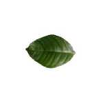
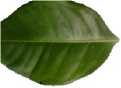
Table 4: Gain percentage from color feature to all features

Recall	Precision		Gain (%)
	Complete	Color
0.0	1.00	1.00	0
0.1	1.00	1.00	0
0.2	0.87	0.87	0
0.3	0.72	0.68	5.88
0.4	0.66	0.62	6.45
0.5	0.60	0.53	13.21
0.6	0.56	0.49	14.29
0.7	0.51	0.43	18.60
0.8	0.48	0.38	26.32
0.9	0.40	0.30	33.33
1.0	0.38	0.27	40.74
Average	0.65	0.60	14.44

(c)

(d)

(e)                                (f)

Fig 6: Various leaf image datasets. (a) original image, (b) rotated, (c) scaled, (d) translated, (e) perspective changed, (f) lighting changed.

Table 4, 5, and 6 show us gain percentage from complete features with every single feature. In table 4, the color feature’s gain-percentage at recall value 0.2 is 0 and it is different from the shape and texture results. The background reason of this occurrence is because there was a different color distribution for the leaf images with index number 3 and 4 inside the database. However, for overall recall values we gained 14.4% in comparison with a single color feature.

Table 5 and 6 are presenting similar trends. From the shape feature result to the complete features result, it is obtained 20.51% of average gain percentage value. From the texture shape result to complete features result, it is obtained 21.48% of average gain percentage value. Generally, all of these results have fulfilled the expectation for this research. Furthermore, the Bayesian weighting formula allowed us to adjust utilization of the features easily. The final similarity can be adjusted whether use only a single feature, double features or complete features.

Table 5: Gain percentage from shape feature to all features          Table 6: Gain percentage from texture feature to all FRATURKS
Recall	Precision		Gain (%)
	Complete	Shape			Recall	Precision		Gain (%)
						Complete	Texture
0.0	1.00	1.00	0
					0.0	1.00	1.00	0
0.1	1.00	1.00	0
					0.1	1.00	1.00	0
0.2	0.87	0.72	20.83
					0.2	0.87	0.78	11.54
0.3	0.72	0.53	35.85
					0.3	0.72	0.50	44.00
0.4	0.66	0.49	34.69
					0.4	0.66	0.47	40.43
0.5	0.60	0.46	30.43		0.5	0.60	0.44	36.36
0.6	0.56	0.43	30.23		0.6	0.56	0.43	30.23
0.7	0.51	0.41	24.39		0.7	0.51	0.40	27.50
0.8	0.48	0.39	23.08		0.8	0.48	0.40	20.00
0.9	0.40	0.35	14.29		0.9	0.40	0.36	11.11
1.0	0.38	0.34	11.76		1.0	0.38	0.33	15.15
Average	0.65	0.56	20.51		Average	0.65	0.56	21.48

Table 7: Image retrieval performances of all datasets

Recall	Precision
	Original	Rotation	Scale	Translation	Perspective	Lighting
0.0	1.00	1.00	1.00	1.00	1.00	1.00
0.1	1.00	0.98	1.00	1.00	1.00	1.00
0.2	0.87	0.82	0.84	0.82	0.79	0.83
0.3	0.72	0.68	0.53	0.42	0.58	0.70
0.4	0.66	0.62	0.45	0.38	0.54	0.64
0.5	0.60	0.55	0.29	0.30	0.45	0.57
0.6	0.56	0.53	0.26	0.27	0.42	0.54
0.7	0.51	0.49	0.18	0.18	0.36	0.48
0.8	0.48	0.45	0.18	0.18	0.33	0.45
0.9	0.40	0.38	0.18	0.18	0.28	0.38
1.0	0.38	0.36	0.18	0.18	0.26	0.36
Average	0.65	0.62	0.46	0.45	0.55	0.63

Recall-Precision Graph

—♦— Original

—■— Rotation

—*— Scale

)( Translation ж Perspective

—•— Lighting

Recall

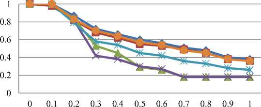
Fig 7: Recall-precision graph for all datasets.

Leaf with Medicinal Functionality Images

Table 7 shows us precision results for all aforementioned datasets. Based on average precision values, the original dataset result occupies the first position. The second position is lighting dataset result, and again we can see, how important the color information for leaf images. The third and fourth positions are occupied by rotation and perspective datasets results. Application of Zernike complex moments method has ensured us to have rotation invariant property. Then, perspective changed in 2-D space was only affected to the leaf shape itself. Even though the shape was affected, color and texture features were still similar, and Bayesian weighting factor will automatically adjust the proper weight from that leaf image.

The fifth and sixth positions are occupied by translation and scale datasets results. From the proposed methods, there are no methods that have complete scale invariant property is the main reason why the scale dataset result was not good. Subsequently, the Dyadic wavelet transformation has translation invariant property, but first process in translation changed dataset was downscaling the image. Therefore, we still faced the same problem with the scale dataset. More visible and understandable results are presented in Fig. 7. It can be seen from the figure that this image retrieval system is very powerful from any rotation, lighting and perspective changes.

• V.    Conclusion

The proposal to add color information to this ornamental leaf images was a correct decision. Instead of utilization of a single feature, utilization of complete features gained much improvement. The Bayesian automatic weighting formula also provided us greatly easiness whether using complete features, single feature or even double features.

Moreover, as seen from the presented results that this image retrieval system had effectiveness especially for original, rotation, and lighting changed datasets. Unfortunately, among three proposed methods, no one has complete scale invariant property, and this issue is a minus point of this research.

• VI.    Future work

Related with the unsatisfying results from scaling and translation datasets, seeking a proper method with scaling invariant property is needed. The convincing candidate is Fourier descriptor method. Further research will involve that method instead of Zernike complex moments. We can adjust Fourier base function to have a scaling invariant as well as rotation invariant properties. From many researches, Fourier descriptor based on centroid distance is a have-to-try method.