Image semantic segmentation using deep learning

Published Online December 2018 in MECS

Image segmentation is one of the fundamental techniques in processing an image. This process includes partitioning model into various segments based on the similarity of the pixel component towards the pixels in the neighbourhood. The pixels that form a pattern which interests further processing techniques is obtained, this makes image segmentation a vital process and enhancement in the quality of segmentation gives better results in image recognition, classification and many other procedures.

Segmentation is one of the most challenging tasks as there are various factors like detection of the edge between the background and the object, segmentation is carried out using multiple techniques such as thresholding, clustering, region-based, edge-based, and using Artificial Neural networks. Clustering is one of the most used and a versatile segmentation technique for large and high-resolution images, and many new approaches have been emerging based on graphs, density clustering, fuzzy clustering etc.

There has been enormous research that is being carried out on automatic image segmentation which is still a difficult task and an alternative method called interactive segmentation is being considered with a considerable user input given to simplify the task. Segmentation of colour images is taking higher importance than grayscale segmentation, and the complexity increases as many new components are to be considered to process an image.

In recent time the best technique to implement segmentation is by using artificial neural networks. Artificial intelligence has given scope for many novel approaches such as using convolution neural networks to map the semantics of an image, other techniques which made a significant contribution to image segmentation using ANN are AlexNet, GoogleNet, ResNet which gave excellent results.

• II.    Proposal Background

We begin the proposal background of Image Segmentation in this section, to make readers have a better understanding of all the image segmentation and object detection research progress and application fields. Artificial intelligence has made a drastic progression in recent years, with several numbers of applications. It has become the primary utility for every researcher for improving unprecedented [1]. This artificial intelligence understands human engagement in solving problems to build an explanatory model. Deep learning which is a subset of Artificial Intelligence has made extensive progress in the fields of computer vision and image processing using neural networks. Neural Networks work in the way the human brain works. They are quite slow when compared to other machine learning algorithms as they need to learn the connection between every given input data. The hardware for deep learning is also progressed with GPUs (Graphics Processing Unit) and TPUs (Tensor Processing Unit) as we need to have enough computational power to run the deep learning algorithms smoothly. Deep Learning techniques include Image feature detection, compression, optimisation, super-resolution(converting low resolution to high resolution) and image generation using several neural network architectures. The most progressed models and equipped for images include forward neural networks, convolutional neural networks and general adversarial neural networks. By this, deep learning can help solve more problems in the fields of Computer Vision and Machine intelligence.

A. Deep Learning - The Model

As discussed above deep learning for image processing is a breakthrough, for image classification and feature detection. These deep learning models include several parameters which need to be trained with many iterations to achieve maximum accuracy and minimum loss. Due to the increase in data and computational power, these become more difficult and time taking to process. The model's efficiencies are defined how well the parameters are tuned for every iteration in the training process and the consistency of the input data. Using the Back Propagation algorithm[5], the model can be made more accurate by sending the loss back through the network and minimising it. The model can be easily defined and architectured with few very minimal restriction.

• III.    Models and Implementation

In the fields of image processing and deep learning, there are several ways in which we use several models for Image Semantic Segmentation. These are developed based on the type of inputs we send in and the consistency of the data. In this section, we will be describing most used models for image feature recognition and segmentation.

• A.    Fully Connected Layers

FCNs take in images of arbitrary sizes and produce the output with efficient learning and inferences. This idea of extending the input size first appeared in Matan et al.[3] which extended the classic LeNet[4] to recognise strings of digits. Prior approaches have used Convolutional Neural Nets for semantic segmentation[6,7,8,9,10,11,12], where each pixel is labelled with a class of its enclosing object or region. FCN is a modified CNN where the last fully connected layers are replaced by convolutional layers with a larger receptive field. Therefore, there are filters everywhere and the decision making layers at the end of a CNN are filters too. It is fully convolutional and therefore capable of predicting the features more accurately since it supports images of any size and also unlike the fully connected layers which no longer care about the spatial arrangement of feature maps but instead focus on classifying the inputs, an FCN continues to detect the features until the last layer.

Convolutional Neural nets are translation invariant, that is they recognise the objects irrespective of where they are placed in images. The convolution, pooling and activation functions operate on the local regions and depend on the relative spatial coordinates. If X i, is the data vector at location (i,j) in a particular layer and y i, for the following layer, then[2]:

where k is kernel size, s is stride, f_ks determines the layer type: matrix multiplication for convolution or average pooling, spatial max for max pooling etc. The above functional form is maintained under the composition:

A network consisting of layers only of this form computes a non-linear filter and is called an FCN. It operates on any input of varying sizes and produces resampled spatial dimensions.

If the loss function is the sum over spatial dimensions in the final layer, l(x;0) = Ey l'(X ij ;9^>) then the gradient will be a sum over the gradients of each of its spatial components.

When a CNN is converted into an FCN, it helps in producing a heat map. Hence, FCNs are the natural choices to implement semantic segmentation on dense and vibrant images. It highlights the objects in the pictures as needed. Ordinary CNN can be used for classification of images to determine the class and for object localisation. Hence, we would be getting limited information whereas an FCN gives a segmented image according to the input image size.

The architecture is the same as that of a CNN with fully connected layers being replaced by convolutional layers. An FCN has kernels in it which produces the feature maps at every layer whose depth depends on the number of kernels. Then this goes to the next convolutional layer and the process repeats. The regularisation or a normalisation layer can be added to the convolutional layers. Also, as the number of convolutional layers increases, the possible interpretations of an image increases as well. The image size reduces as it goes through the pooling layer which allows convolutional layers to capture a more significant part of the object. An upsample layer will enlarge the image by un-pooling, this is termed as deconvolution. Every output has two input images; the first one is processed image from the previous layer: convolution or pooling. The second image is from the pooling layer where the number of outputs is equal to the number of inputs of the correspondent upsample layer and the size of information upsample image is similar to the size of output pooling image. FCN is a combination of both convolutional and deconvolutional networks.

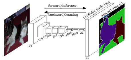
Fig.1. Fully Convolutional Network Architecture for Semantic Segmentation

Disadvantages include a higher computational time since fully connected layers are simpler than convolutional layers which are used in place of them.

• B.    U-Net

Convolutional Neural Networks(ConvNets) is used for several architectures, with different ConvNets architectures. We need to improve the model's structure based on given data and features present in it. In the fields of medical image processing as the output should define localisation of the labels for every pixel, we need to train several images to achieve the highest accuracy which is not possible in the medical science areas. To Overcome this problem Ciresan et al. [14] defined a new architecture to make the process easier by setting up a sliding window to predict the class labels which takes in the pixel regions as matrices or a local neighbourhood. This method has two main drawbacks as it takes more time to compute, and have to run every pixel patches for finding the class labels and memorise them.

To overcome these two problems, Olaf Ronneberger proposed a new kind of convolution neural net architecture which is an extension of the fully connected layer, called U-Net[13]. This architecture only works efficiently for a few types of images, and mostly it is used for medical image processing. In U-Nets using successive layers are increased, where un-sampling operators replace max/avg pooling operations thereby leaving the output image in high resolution. Features from incurring path are connected with the unsampled yield. The core addition to FCN to implement U-Net is it allows the network to pass in the identified elements to the higher level layers of more resolution. In this process, the system might turn into more or less symmetric leaving a U-Shaped Architecture. Though fully connected layers are used in implementing ConvNets, U-Nets don't have any FC layers and only used actual parts of ConvNets, the heat map or segmentation map only has the pixels where the complete image is placed in context.

One of the advantage if using U-Net architecture is that it reduces distortions by learning about the invariance, without recognising the changes in the input image. This is the main reason why these are widely used in medical fields as they reduce distortions in the neighbouring regions and patches.

U-Net Architecture The U-Net architecture is comprised of two parts one on it's left, and one on it's right namely, contracting portion and expansive path respectively. Two 3x3 convolutions are repeated followed by ReLU activation function with two max pooling and two downsampling kernels with stride s = 2. In the right side which is expansive path the sampling was done to the feature map are served by 2x2 convolutions which reduce the number of feature channels to the half these are added with the cropped feature map from the left part i.e,, contracting path wherein again two convolution operation of kernel size 3x3 are done followed by ReLU activation layers. In the last segment, a 1x1 sized convolution operation is done to harmonise every feature vector of 64-component. As we see the figure which is proposed as the official architecture of U-Net[13], it consists of 23 convolution operations. We also require to determine a proper input size so that max operations are implemented with even x and y values.

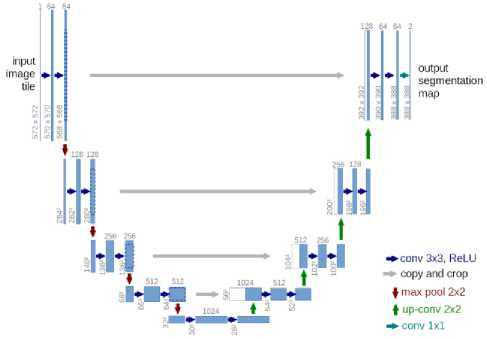
Fig.2. U-Net architecture

The advantage of using U-Net is that it can be applied to real datasets and heavy computation can be made. This Convolutional architecture can be used on agnostic image dimensions which means the input dimensions need not be same all the time. The number of labels and features need not be limited. This U-Net can be trained in graphics processing units for training to be fast. The main disadvantage is that the training time need for tuning the parameters is more when compared to other convolution neural networks architectures. Below are few results that U-Net is applied on and the abnormalities of medical images are found accurately.

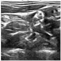
Fig.3. Medical Image Segmentation using U-Net

C.

Deep Lab : Atrous Convolution and Fully Connected CRFs

Recently deepmind implemented a new way to achieve Image Semantic Segmentation which uses convolutional neural networks. This Architecture involves a new type of layers called as Atrous Convolution. The resolution at which feature responses are computed within Deep Convolutional Neural Networks which can be explicitly controlled using Atrous convolution. With these, explicitly the number of filters are iterated without changing any parameters. The second method which finds segments the images are ASPP - Atrous Spatial Pyramid Pooling for scaling multiple objects. These allow in classifying various objects in each scale or level of representation. The third technique that is used is for localising the boundaries of objects in the image by using deep convolutional neural networks and probabilistic programming. This method involves a lot of pooling and downsampling layers this reduces the model to be overfitted following invariance. Initially, deep lab architecture is implemented on PASCAL-Context, PASCAL-Person-Part for image segmentation which gave around 79% accuracy on Image Segmentation [25].

Atrous Convolution Networks for Deep Feature Extraction If the neural network architecture uses many consecutive max pooling and striding layers it reduces the resolution on the images leaving the heatmaps and features and directions of the picture. Including many numbers of layers also increases the training time, however, if the deconvolution layers are applied time and memory will be allocated more efficiently. To tune, this atrous network convolution is implemented which are initially inspired by efficient computation of the undecimated wavelet transform in the “algorithme a trous” scheme from work [26]. If the output features are one dimensional, the equation is represented by [25]

к

Я'] =    л[/ + г.Л.]и>[£]

Where r is the rate parameter corresponding to the stride. When the value of r is one, then it is considered as the particular convolution condition.

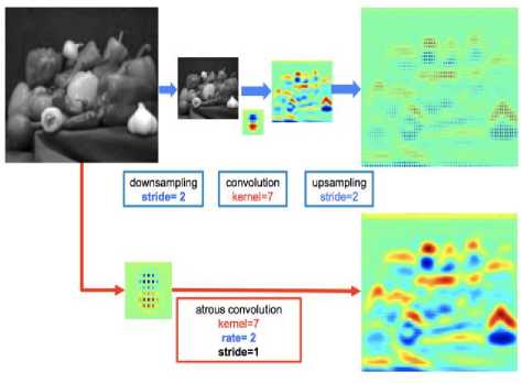
Fig.4. Implementation of Atrous Convolution Networks

The value of stride is mentioned as two, as we keenly observe the above figure the resolution of the image is reduced with the increase in the stride value. A convolution kernel of size seven is used for finding the edges, heat map and the features of the image. Which returned a feature map. Once the feature map has occurred, we use a sampling layer to increase the resolution and highlight the element of the feature map. While in the Atrous structure all the all the kernel and the stride operations are applied proportionally to the rate twice in the neural network which returns a more efficient feature map with higher resolution as seen in the image above.

Atrous Convolutions Architecture These are built upon normal ConvNets which will be expanding their filter's field to increase the resolution of the shirked convoluted image. This architecture can be varied based on the rate at which the dilation happens. When the dilation rate is equal to one, they act like standard convolution neural networks. If the frequency of the atrous convolution increases then the resolution of convolution kernel increases resulting in finding highly segmented objects. When the filter is raised all the empty rows, and columns are filled with zeros creating sparse and then regular convolutions are applied. Initially, the architecture gets dilated with rate 2, and the 3x3 filter will be enlarged with size 5x5. When the frequency is considered as three then the filter changes, it's size from 3x3 to 7x7. One more advantage of the implementation of rate is we will be resulting in a higher context of the image without changing any parameters of the neural network. Also, the rate should be considered concerning the input size if it increases it results in the lower resolution of the feature map with this we can conclude that the efficiency of using atrous network depends on the dilation rate. The downsampling is not contained in the atrous block they are done in the following layers of the network. Below are the segmented images using Atrous Convolutions Architecture by deeplab.

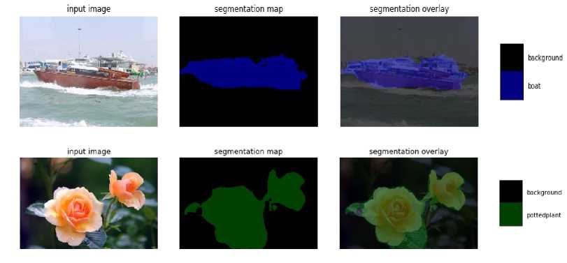
Fig.5. Image Segmentation achieved using Deep Lab models

• D.    SegNet

It represents a deep fully convolutional neural network for semantic pixel-wise segmentation, hence the name SegNet. It comprises an encoder network, a decoder network and a classification layer. Encoder network is where the convolution happens, and the decoder network deconvolves using upsampling and maps the low-resolution features to high-resolution features. The underlying implementation of SegNet lies in upsampling of the low-resolution input feature maps. It is done using the pooling indices which are calculated during the max pooling. The upsamples maps are then convolved with trainable filters to arrive at dense feature maps and hence learning to upsample is not required. Training is carried out end-to-end using Stochastic Gradient Descent (SGD)[18]. SegNet has a vast number of applications like detecting objects in a scene, establishing the relationships among objects during autonomous driving etc.[15]

Deep Neural Network architectures are recently being used in detecting objects in images using pixel-wise labelling, but because sampling and max-pooling reduce the resolution, these days SegNet architectures are gaining momentum. Semantic pixel-wise segmentation is being a lot researched about these days.

Before the arrival of Deep Neural Nets, other algorithms such as Random Forests[19, 20] and Boosting[21, 22] were used to predict the class probabilities of the centre pixel[15]. These are then passed into the CRF(Conditional Random Fields)[21] to improve the accuracy. But the most recent approaches are aiming towards finding the labels for all the pixels as opposed only to the centre pixel. This improves the accuracy, but the thin structured classes are not correctly classified. RGBD classification has also been used, but the common problem is all the features are hand-engineered. Then, CNNs and RNNs have come up and performed well compared to the above techniques, but they are also not able to delineate the boundaries well. VGG16 followed the line consisting of 13 Convolutional layers and 3 Fully-Connected layers. The encoder network is trained, and all the weights are pre-calculated in a VGG16. The decoder network varies between various architectures and classifies each pixel. After that, FCN has arrived which has a vast encoder network but has a smaller decoder network. To avoid this, the step-by-step training process is implemented where each decoder is added progressively until no further changes in the output are detected or until the performance has become saturated. Here, encoder feature maps are reused in the decoder which consumes a lot of memory. A recently proposed Deconvolutional Network[23] uses only the max locations of the feature maps unlike the whole as in FCN[17]. The authors of these architectures have come up with SegNet by removing the fully-connected layers of VGG16 since they make the training complex and also reduce the number of parameters and then appended a decoder network to it.

SegNet helps in mapping the low-resolution features to the input resolution with utmost precision using pixel- wise labelling and semantic segmentation[15]. This mapping produces features for boundary localisation. It also helps in detecting the shapes however small they are; therefore it must retain the boundary details. In larger images where there are more significant objects, a significant number of pixels are confined to a few objects, so smooth segmentations must be produced.

SEGNET Architecture The encoder network is very similar to VGG16[16] by removing the fully connected layers. The significant component of SegNet is a decoder network where there is one decoder corresponding to each encoder; therefore a decoder network has 13 layers. This is done by reusing the max pooling indices since it improves boundary delineation and also reduces the number of parameters. The decoder outputs are then passed into the final classier which gives the class probabilities for each pixel.

The encoder performs convolution to produce feature maps which are then batch normalised[24, 25]. Then a nonlinear ReLU(Rectified Linear Unit) activation function is applied. Following that, max pooling is done using a 2x2 window with a stride of 2, and then it is subsampled by a factor of 2. Before sub-sampling is performed, all the necessary boundary information is captured and stored in the feature maps. This involves storing only the max-pooling indices. The decoder then up samples using the previously stored max-pooling indices which produce sparse feature maps. These are then convolved with filter banks to produce dense feature maps. Then, the outputs are led to a softmax classifier. This finds the class with the maximum probability and returns it at each pixel.

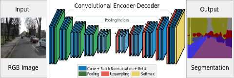
Fig.6. SegNet architecture

Analysis

SegNet is computationally inexpensive compared to the other Neural Nets and has a higher training accuracy. It is also efficient with regards to the inference time and memory.

Below are the results for Image Segmentation when SegNet is used.

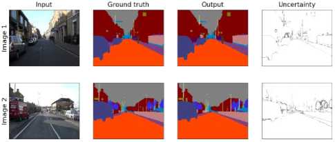
Fig.7. Image Segmentation results for SegNet

• E.    R-CNN To Mask CNN:

The widespread usage of convolution neural networks for object recognition in high-resolution images was first introduced by AlexNet which won the ImageNet in the year 2012. It uses eight layers of which 5 are convolution layers, and the remaining 3 are fully connected networks. AlexNet had the best error rate of 15% whereas others have achieved an error rate of 12%. The use of CNN's in Image segmentation came into prominence with AlexNet showing better accuracy than the SVMs. This inspired Girshick et al. to come up with a new technique called R-CNN.

The goal of this new technique was to detect the objects in an image and define a boundary or regions for that object. The input image is taken, and then it is divided into approximately 2000 areas, each of the areas is then sent into a CNN which is similar to that of AlexNet using caffe[31]. The last layer consists of an SVM to classify the objects, and a linear regression model is run on the model to optimise the regions to precisely fit the purpose to its size. R-CNN successfully segmented the image into the objects, but R-CNN is quite slow as it has to pass every single region into the CNN forward, i.e. approximately 2000 forward passes are required to segment the image into objects completely. The architecture of R-CNN consists of three models, ie model to create regions, model to classify the image and a regression model to optimise the region, and it has to train each model separately. Ross Girshick solved the problems faced by the R-CNN in a new model called Fast R-CNN.

The training and testing time for R-CNN was slow because of burdensome computational requirements, and Fast R-CNN is an approach which was proposed to reduce the Computational time. The input image in R-CNN was divided into regions and then sent into the CNN, but in Fast R-CNN the copy is sent into the network only once, and the computations done on the image are then shared with the sub-regions of the image. This reduces the Training time 3x times and the testing time to 10-100x times. It uses a technique called as Region of interest pooling. The other issue with R-CNN was it uses three different models, and they are trained separately, Fast R-CNN uses a single model which consists of a softmax layer instead of an SVM and parallelly a linear regression layer to optimise the bounding boxes. This way a single network is used to perform the task of three systems.

Fast R-CNN which was an advancement to R-CNN which was computationally quicker than the later but it was not real time fast, it took considerable time when executed on the CPUs. Researches from Microsoft found that the R-CNN uses a selective search method to determine the region proposals, Fast R-CNN uses particular search on the feature map outputted after the image is sent into a CNN. Faster R-CNN uses a method called Region proposal Network(RPNs) which uses the same CNN results obtained by the feature map, instead of using selective search. This way the model has only one CNN to obtain region proposals and classification and region proposals are achieved without using any other algorithm and the cost to compute the region proposals has decreased efficiently.

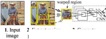
R-CNN Architecture: Regional CNN or R-CNN which was developed with the inspiration by the works carried out on Convolution Neural Networks, revolutionised the way objects are recognised in an image. The input image is divided into many regions using a technique called selective search[27]. It is a process where the image is over-segmented using graph-based segmentation[28] method. Selective search tries to form regions based on the similarity between the adjacent pixels. The over-segmented image is used to form region proposals which are used as inputs for applying Convolution Neural Networks. The regions are wrapped into a box so that they can be sent into the CNN architecture. The neural network used was the 2012 ImageNet winner AlexNet[29] with a slight modification in architecture. The final layer of the architecture consists of an SVM which is used to classify the object.

R-CNN: Regions with CNN features

^| aeroplane? no. |

■► ] person? yes. ]

^ | rvmoni'lor? no. |

4. Classify regions

2. Extract region proposals (~2k)

3. Compute CNN features

Fig.8. R-CNN architecture

The region proposals obtained using selective search are optimised to fit the object to its exact size using a linear regression model which was proposed in DPM[30]. To summarise the architecture of R-CNN, it contains three major parts. First to divide the input image into region proposals, then run each of the region proposals into the CNN layers and using an SVM classify the output. Finally, optimise the regions using a linear regression model.

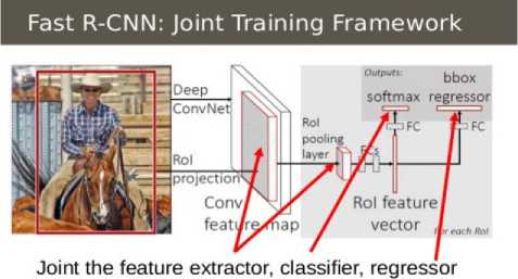
together in a unified framework

Fast R-CNN Architecture: The architecture of Fast R-CNN consists of a RoI pooling layer, many convolution layers where the input image is sent, and a convolution feature map is produced using max-pooling layers. The region proposals obtained using selective search, the region of Interest pooling layer takes in the input and maps any area of interest into a feature map of height H, and width W. each RoI is represented using a tuple with four features(r,c,h,w). The indicate the leftmost corner of the RoI and the height and width of the RoI. The RoI max pooling layer is used to map each subwindow of size h x w to a size of H x W window. RoI pooling layer uses the architecture of SPP nets but with only one pyramid level.

The architecture shows that there is no separate model for classification and regression, Fast R-CNN uses a softmax classifier and a regressor parallelly rather than an SVM and a regressor. There are two outputs to the model one is classification output, and the other is a regressor output. The architecture uses a multitask loss L, and it is jointly trained for both classification and regression.

The loss function for classification is:

The loss function for regression model is L_loc(t^u,v):

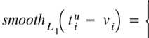
L. (f“,v) =         smooth,(t“ — v

O.5x2, if |x| < 1

A workflow of the fast R-CNN is given as:

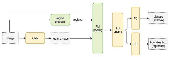
Fig.10.Workflow of R-CNN

Faster R-CNN Architecture: The image is sent into the convolution layers to obtain a feature map which contains all the values, in Faster R-CNN the feature map is used to determine the region proposals by using RPNs. Region proposals are generated by using a sliding window over the feature map. The sliding window location is used to find region proposals, and it predicts multiple region proposals in the same sliding window location which are then fed into a regression model and a classification to obtain objects with a score to each region proposal.

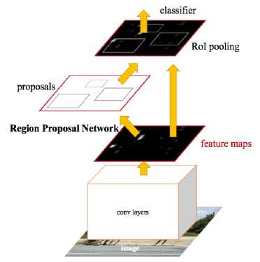
Fig.11. Faster R-CNN architecture

The sliding window with a default size of 3 x 3 aspect ratio is considered, each sliding window predicts region proposals for objects with maximum proposals being k and for default aspect ratio k=9. Each region proposal has an anchor which is centred at the centre of the sliding window. The k anchor boxes are sent into classification and regression layers which output 2k classification scores and 4k regression coordinated which represents the optimised object boundaries.

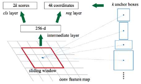
Fig.12. Sliding Window in Faster R-CNN

Mask R-CNN Architecture Mask R-CNN is a technique which uses the concepts of faster R-CNN which classifies objects into bounding boxes. Mask R-CNN is a technique which uses a pixel level identification of an object. The architecture contains the same two-stage architecture of Faster R-CNN where the first stage uses

RPNs to find the region proposals, and in the second stage, it predicts the class of each object and a binary mask which represents 1s where an object is present and 0s where an object is not present.

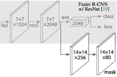
Fig.13. Mask R-CNN architecture

There was a problem which was detected which was when deciding the object boundaries there was a misalignment as the RoI is done on pixels, not on the bounding boxes. Pixel level sensitivity causes the misalignment. To solve this, the authors proposed a technique called RoIAlign. It uses a method called bilinear interpolation[32]. This makes sure the misalignments are not present. Finally, the outputs of the classification and regression models are combined with the masks and pixel level precise image segmentation is done.

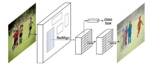
Fig.14. Image Segmentation using Mask R-CNN

Outputs of R-CNN are:

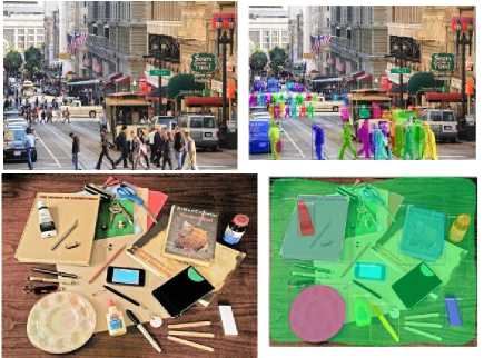
Fig.15. Outputs of R-CNN

• IV. Conclusion

In this work, we discussed Image Semantic Segmentation techniques using deep learning. Using Convolution neural networks, we could achieve the most details that are present in the foreground and background of the images. The best-performed architecture was R-CNN which could quickly identify the objects and segment the images based on the training dataset and the type of objects fed in the dataset. In the fields of medical image processing, the most preferred and used image segmentation is U-Net as it can be iterated over several images for finding and segmenting the images. U-Net is not only used for medical imaging it can also be used for any training dataset of large sizes or inputs. Deep Minds architecture for Semantic Segmentation is used when the segmented image or the feature maps are needed in high resolution, these are applicable in real life scenarios for self-driving cars and detecting all the features of a city. Fully Connected Neural Networks is the underlying architecture for making the multi-channels of an image into segments these architectures helps segmentation in a better understandable way for separating objects from backgrounds of an image using a necessary convolution neural network. We've applied all the deep learning techniques and listed pros and cons for each method including their architectures. We've found that R-CNN is the most efficient way concerning finding the objects in the image and U-Net architecture is widely used for detecting the segments in the picture. All the remaining ConvNet architectures performed well without considering the training time and memory allocation of the neural network.

• [1]    Generative Adversarial Networks: Introduction and Outlook Kunfeng Wang, Member, IEEE, Chao Gou, Yanjie Duan, Yilun Lin, Xinhu Zheng, and Fei-Yue Wang, Fellow, IEEE.

• [2]    Fully Convolutional Networks for Semantic Segmentation, Jonathan Long, Evan Shelhamer UC Berkeley, Trevor Darrell.

• [3]    O. Matan, C. J. Burges, Y. LeCun, and J. S. Denker. Multi- digit recognition using a space displacement neural network. In NIPS, pages 488–495. Citeseer, 1991.

• [4]    Y. LeCun, B. Boser, J. Denker, D. Henderson, R. E. Howard, W. Hubbard, and L. D. Jackel. Backpropagation applied to handwritten zip code recognition. In Neural Computation, 1989.

• [5]    Learning representations by back-propagating errors David E. Rumelhart, Geoffrey E. Hinton & Ronald J. Williams, Nature Volume 323, pages 533–536 (09

October 1986)

• [6]    F. Ning, D. Delhomme, Y. LeCun, F. Piano, L. Bottou, and P. E. Barbano. Toward automatic phenotyping of developing embryos from videos. Image Processing, IEEE Transactions on, 14(9):1360–1371, 2005.

• [7]    D.C.Ciresan,A.Giusti,L.M.Gambardella,and J.Schmid-huber. Deep  neural  networks  segment neuronal

  membranes in electron microscopy images. In NIPS, pages 2852–2860, 2012.

• [8]    C. Farabet, C. Couprie, L. Najman, and Y. LeCun. Learning hierarchical features for scene labeling. Pattern Analysis and Machine Intelligence, IEEE Transactions on, 2013.

• [9]    P. H. Pinheiro and R. Collobert. Recurrent convolutional neural networks for scene labeling. In ICML, 2014.

• [10]    B. Hariharan, P. Arbela ́ez, R. Girshick, and J. Malik. Simultaneous detection and segmentation. In European Conference on Computer Vision (ECCV), 2014.

• [11]    S. Gupta, R. Girshick, P. Arbelaez, and J. Malik. Learning rich features from RGB-D images for object detection and segmentation. In ECCV. Springer, 2014.

• [12]    Y. Ganin and V. Lempitsky. N4-fields: Neural network nearest neighbor fields for image transforms. In ACCV, 2014.

• [13]    U-Net: Convolutional Networks for Biomedical Image Segmentation Olaf Ronneberger, Philipp Fischer, Thomas Brox arXiv:1505.04597

• [14]    Ciresan, D.C., Gambardella, L.M., Giusti, A., Schmidhuber, J.: Deep neural networks segment neuronal membranes in electron microscopy images. In: NIPS. pp. 2852–2860 (2012)

• [15]    SegNet:  A Deep Convolutional Encoder-Decoder

Architecture for Image Segmentation, Vijay Badrinarayanan, Alex Kendall, Roberto Cipolla, Senior Member, IEEE.

• [16]    K. Simonyan and A. Zisserman, “Very deep convolutional networks for large-scale image recognition,” arXiv preprint arXiv:1409.1556, 2014.

• [17]    Long, E. Shelhamer, and T. Darrell, “Fully convolutional networks for semantic segmentation,” in CVPR, pp. 3431–3440, 2015.

• [18]    L. Bottou, “Large-scale machine learning with stochastic gradient de- scent,” in Proceedings of COMPSTAT’2010, pp. 177–186, Springer, 2010.

• [19]    J. Shotton, M. Johnson, and R. Cipolla, “Semantic texton forests for image categorization and segmentation,” in CVPR, 2008.

• [20]    G.Brostow,J.Shotton,J.,andR.Cipolla,“Segmentationandre cognition using structure from motion point clouds,” in ECCV, Marseille, 2008.

• [21]    P. Sturgess, K. Alahari, L. Ladicky, and P. H.S.Torr, “Combining appear- ance and structure from motion features for road scene understanding,” in BMVC, 2009.

• [22]    L. Ladicky, P. Sturgess, K. Alahari, C. Russell, and P. H. S. Torr, “What, where and how many? combining object detectors and crfs,” in ECCV, pp. 424–437, 2010.

• [23]    H. Noh, S. Hong, and B. Han, “Learning deconvolution network for semantic segmentation,” in ICCV, pp. 1520– 1528, 2015.

• [24]    S. Ioffe and C. Szegedy, “Batch normalization: Accelerating deep network training by reducing internal covariate shift,” CoRR, vol. abs/1502.03167, 2015.

• [25]    DeepLab: Semantic Image Segmentation with Deep Convolutional Nets, Atrous Convolution, and Fully Connected CRFs Liang-Chieh Chen, George Papandreou, Senior Member, IEEE, Iasonas Kok

• [26]    M. Holschneider, R. Kronland-Martinet, J. Morlet, and P. Tchamitchian, “A real-time algorithm for signal analysis with the help of the wavelet transform,” in Wavelets: Time-Frequency Methods and Phase Space, 1989, pp. 289–297

• [27]    J. Uijlings, K. van de Sande, T. Gevers, and A. Smeulders. Selective search for object recognition. IJCV, 2013

• [28]    Pedro F. Felzenszwalb, Efficient Graph-Based Image Segmentation, Lecture notes in computer science, Artificial Intelligence Lab, Massachusetts Institute of Technology

• [29]    A. Krizhevsky, I. Sutskever, and G. Hinton. ImageNet classification with deep convolutional neural networks. In NIPS, 2012.

• [30]    P. Felzenszwalb, R. Girshick, D. McAllester, and D. Ramanan.Object detection with discriminatively trained part based models. TPAMI, 2010.

• [31]    Y. Jia, E. Shelhamer, J. Donahue, S. Karayev, J. Long, R. Girshick, S. Guadarrama, and T. Darrell. Caffe: Convolutional architecture for fast feature embedding. In Proc. of the ACM International Conf. on Multimedia, 2014.

• [32]    M. Jaderberg, K. Simonyan, A. Zisserman, and K. Kavukcuoglu. Spatial transformer networks. In NIPS, 2015.