Image training, corner and FAST features based algorithm for face tracking in low resolution different background challenging video sequences

Автор: Ranganatha S., Y. P. Gowramma

Журнал: International Journal of Image, Graphics and Signal Processing @ijigsp

Статья в выпуске: 8 vol.10, 2018 года.

Бесплатный доступ

We are proposing a novel algorithm for tracking human face(s) in different background video sequences. We have trained both face and non-face images which help in face(s) detection process. At first, FAST features and corner points are extracted from the detected face(s). Further, mid points are calculated from corner points. FAST features, corner points and mid points are combined together. Using the combined points, point tracker tracks face(s) in the frames of the video sequence. Standard metrics were adopted for measuring the performance of the proposed algorithm. Low resolution video sequences with challenges such as partial occlusion, changes in expression, variations in illumination and pose took part while testing the proposed algorithm. Test results clearly indicate the robustness of the proposed algorithm on all different background challenging video sequences.

Еще

Tracking human face(s), Different background, Video sequences, FAST features, Corner points, Low resolution

Короткий адрес: https://sciup.org/15015987

IDR: 15015987 | DOI: 10.5815/ijigsp.2018.08.05

Текст научной статьи Image training, corner and FAST features based algorithm for face tracking in low resolution different background challenging video sequences

Video processing has large scope for research activities in computer vision. Problems based on face detection, tracking and recognition comes under video processing. Face tracking in low resolution different background video sequences is very crucial because of broad range of commercial and law imposition applications in the real life situation.

A. Face Tracking Overview

Face tracking involves three major steps. In the beginning, face(s) needs to be detected; which indicates that faces are the region of interest (ROI) in face(s) tracking setup. Next, features are selected and isolated from the face(s) detected. Few searching features need to be selected, as features selected increase processing speed by minimizing the computational space. Tracking algorithms are classified as intensity-based, feature-based, area-based and curve/edge based [1]. Algorithms based on features can be classified further into three divisions according to the type of feature selected. The divisions are as follows. 1). Regional-feature-based algorithms comprise corner points, curve chunks and line slices as features. 2). Universal-feature-based algorithms include areas, centroids, colors and perimeters as features. 3). Graph-feature-based algorithms consist of geometric similarities among features and many type of distances as features. Finally, based on the features isolated from ROI, face tracking step tracks face(s) in a video sequence.

B. Different Background and Issues

Video sequences are said to have different background if they are captured using,

1. Unmoving camera and moving face(s),
2. Moving camera and unmoving face(s),
3. Moving camera and moving face(s).

Specific algorithms are unavailable to track face(s) in all the above said categories of video sequences. Face(s) tracking in different background video sequences is challenging due to the following possible issues.

1. Difficult to track face(s) due to the challenges such as partial occlusion (helmet, beard, spectacle
2. Difficult to track face(s) in all the frames of the video sequences with difficult/cluttered background.
3. Chances of tracking non-face(s) in background posters, mirrors and in other locations of the frame.
4. Difficult to track face(s) in improperly captured indoor and outdoor short/long video sequences.
5. Difficult to track face(s) in case of video sequences captured using moving camera with unmoving face(s) and moving camera with moving face(s) categories due to the change in background from frame to frame.

etc.), sudden change in pose, expression and illumination.

Proposed algorithm is able to track face(s) in all the three categories of video sequences as mentioned above and tackles the possible issues very efficiently.

C. Work Description and Organization of the Paper

Exactly 19531 images are classified as either face (positive) or non-face (negative). Classified images assist during face(s) detection step. ROI regions are obtained during this process. Both single and multiple faces are detected and the face(s) need not to be part of starting frame/image in the video sequence. Dilation and erosion [2] operations are applied on the detected face(s) to obtain borders. FAST (Features from Accelerated Segment Test) features [3] and Harris corner points [4] are extracted from ROI and borders. Mid points are calculated for the Harris corner points extracted. FAST features, Harris corner points and mid points are combined together. To keep track of face(s), face tracking step looks at the combined points in the frames of the video sequence. If FAST feature points fail to contribute during tracking then corner points assist the process and the reverse is also true. Standard metrics helped in assessing the attainment of our proposed algorithm with other five similar algorithms of recent times. Proposed algorithm is being tested on low resolution different background challenging video sequences from three different sources. Proposed algorithm tackles the challenges [36] such as partial occlusion, expression, illumination and pose appearing in the frames of the video sequences.

The remaining sections of this paper are planned as mentioned in the following lines. Section 2 incorporates literature works that were referred as well as adopted during the preparation of current (proposed) algorithm. Section 3 includes image training description; training, detection and tracking methods; related mathematics and time complexity. Section 4 houses various metrics which assist in measuring the performance of the algorithms. Section 5 contains detailed results and graphs of six algorithms (including proposed algorithm) for different video sequences. Lastly, section 6 comprises conclusion of the paper; and talks about the works to be done further.

II. Related Works

Face(s) detection can be performed either using existing algorithms or by image training. Viola-Jones algorithm [5, 6] is an efficient face(s) detection framework available till date. Viola and Jones have trained the algorithm to detect frontal posed face(s) appearing in the first frame. Detection of face(s) having other orientations require additional training; and for detecting face(s) appearing in other frames, algorithm needs to be modified. The ToolboxTM of Computer Vision System supports Viola-Jones algorithm [7] for face detection in image and video. Elena Alionte et al. [8] have developed a face detector based on Viola-Jones framework. The detector was configured to use the specification of XMLFILE input file, created using trainCascadeObjectDetector function.

Image pre-processing is very crucial due to camera orientation, illumination difference and noise. Wiener filter is one of the most powerful noise removal approach [9], which has been used in several applications. Dilation and erosion are morphological operations [2] that are dual to each other i.e. erosion operation shortens foreground, and expands background; dilation operation expands foreground and shortens background.

E. Rosten et al. [3] have presented a method by integrating point and edge based tracking approaches. They showed how learning improves the performance of tracking based on features. Finally, to improve performance during real-time, they introduced FAST features that perform feature detection of full-frame at 400Hz. The system is able to track average errors of 200 pixels.

An object consists of three regions: 1). Flat: No transition in any direction, 2). Edge: No transition in edge direction, and 3). Corner: Major transition in all directions. To elaborate the regions containing isolated and texture features, C. Harris et al. [4] have adopted a detector by combining corner and edge regions. The performance of the detector is shown to be good on natural imagery. Mahesh et al. [10] have suggested a method to detect feature points, and compared it with KLT [11-13], conventional Harris [4] and FAST features [3]. They claim that, their approach has good repeatability rate compared to remaining detectors.

KLT is a point tracker, which is due to the works of kanade et al. [11-13]. Lucas and Kanade [11] have presented a technique for image registration using Newton-Raphson type of iteration. This technique can be universalized to manage scaling, shearing and rotation; and found to be appropriate for usage in a stereo vision system. Tomasi and Kanade [12] have answered the question on how to determine the best fitted feature window for tracking; additionally, they have also addressed occlusion detection issue. The experiment indicates that the performance of their tracking algorithm is acceptable. Shi and Tomasi [13] have introduced an optimal algorithm to select the features, formulated on the basis of working of the tracker; and a method for detecting occlusions, disocclusions, and the features not corresponding to the points. These methods extended the previous Newton-Raphson type of searching; and found to be invariant under affine transformations.

Bradski [14] modified mean shift [15] algorithm to work with changing color distributions of video image sequences. The altered algorithm became familiar as CAMSHIFT. It is one of the best motion tracking algorithm based on chromatic values implemented till date.

Ranganatha S et al. [16] have developed an algorithm by fusing corner points and centroid with KLT. Test results indicate that, fused algorithm work better in most of the videos compared to KLT alone. But, the algorithm is capable of tracking only single face in video sequences captured using unmoving camera and moving face(s) category. Ranganatha S et al. [17] have developed another algorithm by integrating CAMSHIFT [14] and Kalman filter [18-20]. Kalman filter minimizes noise and updates current frame information to the next frame in video. Due to this, their integrated algorithm work robust compared to CAMSHIFT algorithm alone. Like their previous approach, this algorithm is also unable to track face(s) in moving camera with unmoving face(s) and moving camera with moving face(s) video sequence categories. Ranganatha S et al. [1] have developed one more algorithm for face tracking in video sequences using BRISK (Binary Robust Invariant Scalable Keypoints) feature points [21]. This algorithm tracks both single and multiple faces in all categories of different background video sequences. The authors have also developed novel metrics for measuring performance; tested their algorithm on a variety of video sequences and tabulated the results.

Table 1. Statistics of face images trained.

Sl No.	Database	No. of Images Trained	Resolution (Pixels)
01.	Caltech [22]	1212	36 x 36
02.	Faces94 [23]	46	180 x 200
03.	ORL [24]	400	92 x 112
04.	Taiwan [25]	1258	640 x 480
05.	Yale [26, 27]	826	195 x 231

Table 2 below tabulates the number of non-face images of 3 databases trained.

Table 2. Statistics of non-face images trained.

Sl No.	Database	No. of Images Trained
01.	Caltech [22]	132
02.	101_ObjectCategories [28, 29]	2013
03.	256_ObjectCategories [30]	13644

Each non-face image has different resolution. Training of more non-face images increases the probability of face(s) detection. Hence, we trained more negative than positive images. Some of the subject categories of nonface images trained are numerous animals, household items, vehicles, plants and flowers, electronic gadgets, indoor and outdoor scenes etc. to name a few.

Few of the face (positive) and non-face (negative) image samples being trained are included in Fig.1 and Fig.2 respectively. Fig.3 summarizes the image training phase; and a brief image training procedure is enclosed in Algorithm 1 below.

III. Methodology

This section houses three subsections A, B and C.

A. Image Training

Trained images help in face(s) detection step. Using trainCascadeObjectDetector trainer [8], we have trained 19531 images; out of which 3742 were faces (positive images) of 5 face databases and 15789 were non-faces (negative images) of 3 databases. Face images being trained possess various challenges and belong to different subject categories such as occlusion, padding, pose, expression and illumination. Table 1 shows statistics of 3742 face images trained.

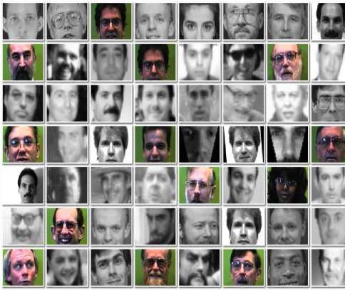
Fig.1. Face (positive) image samples trained.

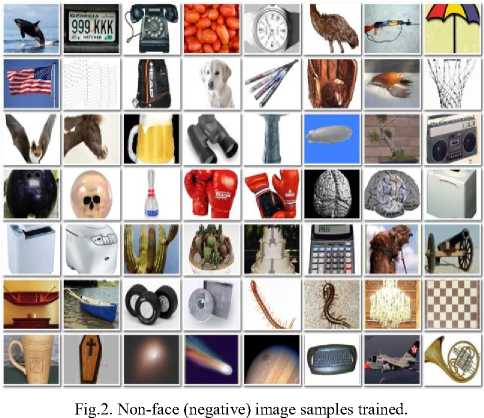
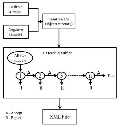
Fig.3. Summary of image training phase.

B. Face(s) Tracking

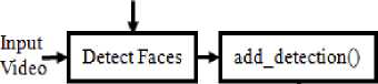
Face(s) tracking system architecture is summarized in Fig.4 below.

Trained XML File

Generate

Points

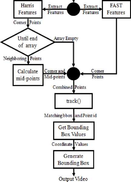
Fig.4. Face(s) tracking system architecture.

Face(s) tracking phase includes different functions. All these functions are housed in Algorithm 2 below.

Algorithm 1: Image Training Phase

1. Collect positive and negative samples in at least 1:2 ratio.
2. Load all positive sample images and manually select ROI regions in each image.
3. Load all ROI values to a variable positiveInstances, and save the collections as a .mat file.
4. Load .mat file and positiveInstances.
5. Store the path of positive samples folder to a
6. Store the path of negative samples folder to a
7. Call the in-built function

variable.

trainCascadeObjectDetector by passing parameters such as xml file name to be created, positive samples path, negative samples path, false alarm rate, and number of cascade stages.

Algorithm 2: Face(s) Tracking Phase

1. Function main()

1. Use trained xml file as parameter to vision.CascadeObjectDetector.
2. Select a video to apply the algorithm.
3. Calculate the size of each frame required to initialize video player.
4. Initialize a variable bbox=[] to store the detected face co-ordinates.
5. Initialize keep_running=true.
6. While keep_running

1. While isempty(bbox)

a. F1=Read each frame.
b. F2=Convert RGB frame to grayscale.
c. F3=Apply wiener filter to F2.
d. Detect the face using the detector; store the location or co-ordinates of the face detected.
2. If ~isempty(bbox)

End

a. add_detection(F1,bbox).

Else

b. track(F1).
3. Draw a rectangular box for bbox values.
2. Function add_detection(frame,bbox)

End

1. If isempty(boxid) // for new face

1. F4=Convert the frame into binary using im2bw.
2. P1=Extract FAST features from the region of
3. P2=Extract Harris corner points from ROI of F4.

interest (ROI) of F4.

Repeat

a. Calculate the midpoints between two consecutive points of P1.
4. Combine all the 3 points (P1, P2, midpoints) and pass it to the KLT tracker to track the faces using these points.

Until Midpoint is calculated between all the consecutive points of P1 array.

Else // if ~isempty(boxid) i.e. existing face

1. F5=Convert the frame into binary using im2bw.
2. P3=Extract FAST features from the region of
3. P4=Extract Harris corner points from ROI of F5.
4. Calculate the midpoints between every two consecutive points of P3; continue this step until all the midpoints are calculated.
5. Combine all the 3 points (P3, P4, midpoints) and pass it to the KLT tracker to track the faces using these points.
3. Function track(frame)

interest (ROI) of F5.

End

1. If bboxes!=empty

1. Call add_detection().

Else

1. Get points and pointId’s from KLT tracker.
2. Get boxId’s and find unique pointId’s.
3. Fill bbox with zero’s.

Repeat

a. Get points with matching pointId’s of all the faces present in the frame.
b. generateNewboxes(points).
2. Draw rectangle around the face region detected; and take next frame.
4. Function generateNewboxes(points)
5. Function obtainBBox(points)

Until all the detected faces have bounding-boxes in that frame.

End

1. X₁=lower-bound(points-off(:,1)).
2. X =upper-bound(points-off(:,2)).
3. Y 1 =lower-bound(points-off(:,1)).
4. Y =upper-bound(points-off(:,2)).
5. bbox=[X₁,Y₁,width,height].
6. Return bbox values.

C. Mathematical Computations and Time Complexity

The mathematical computations of the proposed algorithm are mentioned below.

Area > 0.2* BBox ( width ) * BBox ( height ) . (1)

Where BBox =Bounding Box. To find identical bounding box, calculate area of bounding boxes using equation (1).

Xt = minimum (points (:, 1)),

X2 = maximum (points (:,2)), Y, = minimum (points (:, 1)),

Y = maximum (points (:, 2))

Equation (2) can be used to draw BBox i.e. Bounding Box around the face region.

Bounding Box Region = [X,, Y, X2 - X,, Y - Y ]. (3)

Equation (3) determines the bounding box region. The four arguments of the equation are described as X = X-

Coordinate, Y = Y-Coordinate, X ₂ — X j = Width value, and Y — Y = Height value.

(BoxScores < 3) — 0.5 < minimumBoxScore.(4)

We eliminate bounding box contents when they are not tracked any more, if equation (4) results in true.

Mid ( x, y ) = f x^, y^ ).(5)

V 7 ( 22

Equation (5) computes the mid-point between two consecutive points p 1 ( x , y ) and p 2 ( x ₂, y ₂) .

Time complexity of our proposed algorithm can be estimated as follows:

1. main() function takes O ( _n ² ) i.e. quadratic time.
2. Time taken by add_detection() function is linear in nature i.e. O ( n ) + O ( n ) = 2O ( n ) .
3. Growth of track () function is linear again i.e.
4. generateNewboxes () function takes a constant time of O (1).
5. Similarly, obtainBBox () function belongs to a constant time of O (1) .

2 O ( n ) + O (n) = 3 O ( n ) .

Finally, overall time complexity of current algorithm is the addition of complexities of five functions i.e. T ( overall ) = O ( n ² ) + 2 O ( n ) + 3 O ( n ) + O ( 1 ) + O ( 1 ) ■

After simplifying,

T ( overall ) = O ( n ² ) + 5 O ( n ) + 2 O ( 1 ) ■ By neglecting linear and constant terms, overall time complexity can be approximated as mentioned below.

T ( overall ) ® O ( n ² ) ■

Negative ( n ) situation arises when human vision identifies facial region(s) in the frame but algorithm fails to find the ROI (facial region). Finally, True Negative ( p ) situation arises when both human vision as well as algorithm detects the absence of facial region in the frame and both rejects it, as no ROI is detected. Once after the algorithm detects the presence of ROI in a frame, it plots a bounding box around it; and the computation of new metrics are based on the metrics defined above. We now discuss eight metrics that can be derived from the confusion matrix [35].

A. Recall/True Positive Rate ( T )

It is the measure of positive scenarios by both human vision and algorithm with respect to actual positive scenarios that are identified by human vision. So, T can be defined as follows:

IV. Metrics

The performance of the proposed algorithm has been measured using standardized formulas such as Precision, Recall and F-Measure of ROC [34]; and with the help of concepts in the ROC analysis [35]. The ROC analysis is based upon the confusion matrix, using which several common performance metrics can be extracted such as True Negative Rate, False Negative Rate, Accuracy, and so on.

False Positive

Negative

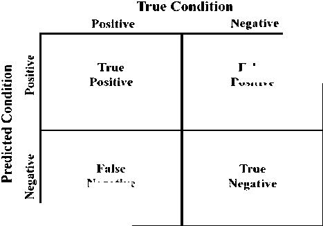
Fig.5. Confusion matrix.

Fig.5 represents confusion matrix [35] that states the relation between true condition (human vision) with respect to predicted condition (algorithmic). This matrix classifies 4 metrics based on the conditions for performance evaluation: True Positives, True Negatives, False Positives and False Negatives. We next discuss about these metrics and compute other metrics from these.

In this paper, ROI focus is on facial region; so, metrics and computations are based on the same ROI. True Positive ( ф ) condition arises when both human vision and algorithm detects the facial region in the particular frame. Likewise, False Positive ( ф ) condition arises when human vision does not identify the ROI predicted by the algorithm as facial region. Similarly, False

True Positive . ф t =---------------------- i.e. t =------■ (6)

Condtion Positive ф + n

B. Precision/Positive Predictive Value ( Z )

It is the measure of positive scenarios by both human vision and algorithm with respect to actual positive scenarios that are identified by algorithm. So, Z can be defined as follows:

True Positive

Predicted Condition Positive

Ф i.e. ^ = 1----. (7)

^ф + ф

C. True Negative Rate ( V )

It is the measure of negative scenarios by both human vision and algorithm with respect to actual negative scenarios that are identified by human vision. So, V can be defined as follows:

True Negative . p

V = --------------------- i.e. v =------ . (8)

Condition Negative p + ф

D. Negative Predictive Value ( Z )

It is the measure of negative scenarios by both human vision and algorithm with respect to actual negative scenarios that are identified by algorithm. So, Z can be defined as follows:

Z =---- ...■,.,----

Predicted Condition Negative i.e. Z = . (9)

P + n

E. Miss Rate/False Negative Rate ( V )

It is the measure of negative scenario by algorithm but positive scenario observed by human vision with respect to actual positive scenarios that are identified by human vision. So, V can be defined as follows:

determines the test’s accuracy. F1 Score reaches 1 for perfect precision and recall reaches 0 in the worst case. So, B can be defined as:

False Negative v =---------------

Condition Positive

i.e. v = ^^ . (10)

П + ф

Precision x Recall

B = 2l

V Precision + Recall

I 5 x T I

i.e. B = 2l ------ I. (13) V 5 + T )

F. Fall-Out/False Positive Rate ( 9 )

It is the measure of negative scenario by human vision but positive scenario observed by algorithm with respect to actual negative scenarios that are identified by human vision. So, 9 can be defined as follows:

„ False Positive ф

9 = i.e. 9 = -1-

Condition Negative ф +

G. Accuracy ( A )

It is the measure of both positive and negative scenarios agreed by human vision as well as algorithm with respect to actual population in the confusion matrix. So, A can be defined as follows:

True Positive + True Negative

Total Population of Matrix

■ л ф + P i.e. A =-----------------.

ф + p + ф + n

H. F1 Score (B)

The measure which joins precision ( 5 ) with recall ( T ) is termed harmonic mean between both precision as well as recall. In analysis, a F1 Score or F-Measure

Using the computed values of ф , p , ф and П , equations (6) to (13) compute T , 5 , у , Z , V , 9 , A and B respectively.

V. Results and Analysis

The algorithm has been tested for 50 low resolution different background challenging video sequences obtained from the following.

1. YouTube Celebrities database [31].
2. VidTIMIT database [32].
3. MathWorks videos [33].

We have compared the current (proposed) algorithm with five other similar (and robust) algorithms developed in recent times. The five algorithms are KLT [11-13], CAMSHIFT [14], Algorithm* [1], Algorithm# [16] and Algorithm^ [17]. These algorithms were tested with all the videos that are considered for the computation; out of which, results of 15 videos have been tabulated for reference purpose. Some of the frames of the 15 video sequences containing the face(s) detected and tracked are shown in Fig.6 below.

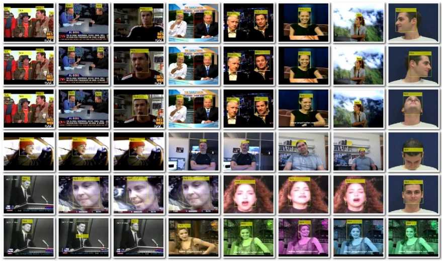
Fig.6. Results obtained after testing the proposed (current) algorithm with 15 low resolution different background challenging videos.

0060_01_005_al_gore.avi	as	video 3,
0092_02_013_al_gore.avi	as	video 4,
0193_01_004_alanis_morissette.avi	as	video 5,
0245_03_005_anderson_cooper.avi	as	video 6,
0277_01_007_angelina_jolie.avi	as	video 7,

0286_01_016_angelina_jolie.avi as video 8, 0358_03_002_ashley_judd.avi as video 9, 0673_01_004_gloria_estefan.avi as video 10, 0689_02_006_gloria_estefan.avi as video 11, 1604_01_012_ronald_reagan.avi as video 12, mcem0_head.mpg as video 13, tilted _face.avi as video 14, and visionface.avi as video 15.

Table 3. Results of current (proposed) algorithm against different video sequences.

VIDEO	No. of Frames	Time (sec)	TP	TN	FP	FN	TPR	TNR	PPV	NPV	FNR	FPR	ACC	F1 Score
Video 1	28	6.8	28	0	0	0	1	0	1	0	0	0	1	1
Video 2	47	5.6	47	0	0	0	1	0	1	0	0	0	1	1
Video 3	62	6.2	62	0	0	0	1	0	1	0	0	0	1	1
Video 4	106	6.8	106	0	0	0	1	0	1	0	0	0	1	1
Video 5	23	6.1	23	0	0	0	1	0	1	0	0	0	1	1
Video 6	148	9.9	148	0	0	0	1	0	1	0	0	0	1	1
Video 7	12	5.8	12	0	0	0	1	0	1	0	0	0	1	1
Video 8	186	8.5	186	0	0	0	1	0	1	0	0	0	1	1
Video 9	29	6.3	29	0	0	0	1	0	1	0	0	0	1	1
Video 10	67	6.2	67	0	0	0	1	0	1	0	0	0	1	1
Video 11	31	6.4	31	0	0	0	1	0	1	0	0	0	1	1
Video 12	280	10.1	280	0	0	0	1	0	1	0	0	0	1	1
Video 13	365	25.7	365	0	0	0	1	0	1	0	0	0	1	1
Video 14	413	41.4	413	0	30	0	1	0	0.93	0	0	1	0.93	0.96
Video 15	65	10.9	65	0	0	0	1	0	1	0	0	0	1	1

The videos are tested for the performance metrics that are discussed in the previous section. The metrics are used as abbreviations such as ‘TP’ for True Positive, ‘TN’ for True Negative, ‘FP’ for False Positive, ‘FN’ for False Negative, ‘TPR’ for True Positive Rate, ‘TNR’ for True Negative Rate, ‘PPV’ for Positive Predictive Value, ‘NPV’ for Negative Predictive Value, ‘FNR’ for False Negative Rate, ‘FPR’ for False Positive Rate and ‘ACC’ for Accuracy. ‘Time’ is in terms of seconds; and ‘-’ in all the tables represent Fail/False state, indicating the absence of faces or failing of tracking face(s) in that video sequence.

The performance metrics for the current (proposed) algorithm are calculated by considering 15 videos and the outcomes are tabulated in Table 3 above. In the table we can observe that out of 15 video sequences considered for testing, only one video has slight deviation from perfect result; that is due to tilting of the face, variations and disturbances in the video sequence.

The performance metrics for Algorithm* [1] are calculated by considering 15 videos and the outcomes are tabulated in Table 4. In the table we can observe that there are various fail states in results computed using 15 video sequences; it is because of occluded faces, no proper posed face in first frame and so on. We can also note that time is computed, indicating that Algorithm* [1] has been executed but failed in detection and tracking of ROI. Along with the failed details, results of other cells for different metrics are also poorer compared to the results of the algorithm presented in this paper.

The results of performance metrics for Algorithm# [16] are tabulated in Table 5. We can observe that there are various false conditions, due to the same reasons as mentioned in the previous paragraph for Algorithm * [1]. Comparatively, there are lesser variations in the results of performance metrics. The drawback of this algorithm is, it is limited to track only a single face. In case if multiple faces are detected, the Algorithm# [16] shows exceptions.

Table 6 tabulates the results of performance metrics for KLT algorithm [11-13]. The results indicate that KLT algorithm is similar to Algorithm#; and suffers from the same issues as the later. KLT algorithm takes more time than that of Algorithm# for computation and obtaining of results; and it fails at many places where Algorithm# works better. But, both KLT and Algorithm# fail in the computation of multiple faces.

Table 7 shows the results of testing the video sequences using CAMSHIFT algorithm [14]. CAMSHIFT is different from all other previous algorithms due to the fact that it is based on color/HUE schema of the videos given as input to the algorithm. CAMSHIFT gives rise to more false detections as every frame is sensitive to color and illumination changes in the video sequence; which causes variations in the bounding box, leading to false detections.

Table 8 shows the results of testing the video sequences using Algorithm^ [17]. This algorithm is similar to CAMSHIFT; but, it is better in few aspects of computation and time taken for computation.

Table 4. Results of Algorithm* for different video sequences.

VIDEO	No. of Frames	Time (sec)	TP	TN	FP	FN	TPR	TNR	PPV	NPV	FNR	FPR	ACC	F1 Score
Video 1	28	1.7	-	-	-	-	-	-	-	-	-	-	-	-
Video 2	47	8.3	44	0	0	3	0.94	0	1	0	0.06	0	0.94	0.97
Video 3	62	2.7	-	-	-	-	-	-	-	-	-	-	-	-
Video 4	106	3	-	-	-	-	-	-	-	-	-	-	-	-
Video 5	23	2.9	23	0	0	0	1	0	1	0	0	0	1	1
Video 6	148	49.5	148	0	0	0	1	0	1	0	0	0	1	1
Video 7	12	5	12	0	0	0	1	0	1	0	0	0	1	1
Video 8	186	10.9	186	0	0	0	1	0	1	0	0	0	1	1
Video 9	29	4.6	22	0	0	7	0.76	0	1	0	0.24	0	0.76	0.86
Video 10	67	2.7	-	-	-	-	-	-	-	-	-	-	-	-
Video 11	31	7.5	31	0	0	0	1	0	1	0	0	0	1	1
Video 12	280	6	-	-	-	-	-	-	-	-	-	-	-	-
Video 13	365	80.6	365	0	0	0	1	0	1	0	0	0	1	1
Video 14	413	112.8	413	0	35	0	1	0	0.92	0	0	1	0.92	0.96
Video 15	65	15.8	58	0	0	7	0.89	0	1	0	0.11	0	0.89	0.94

Table 5. Results of Algorithm# for different video sequences.

VIDEO	No. of Frames	Time (sec)	TP	TN	FP	FN	TPR	TNR	PPV	NPV	FNR	FPR	ACC	F1 Score
Video 1	28	-	-	-	-	-	-	-	-	-	-	-	-	-
Video 2	47	5	47	0	0	0	1	0	1	0	0	0	1	1
Video 3	62	-	-	-	-	-	-	-	-	-	-	-	-	-
Video 4	106	-	-	-	-	-	-	-	-	-	-	-	-	-
Video 5	23	3.1	23	0	0	0	1	0	1	0	0	0	1	1
Video 6	148	-	-	-	-	-	-	-	-	-	-	-	-	-
Video 7	12	4.1	12	0	0	0	1	0	1	0	0	0	1	1
Video 8	186	9.8	186	0	0	0	1	0	1	0	0	0	1	1
Video 9	29	3.3	29	0	0	0	1	0	1	0	0	0	1	1
Video 10	67	-	-	-	-	-	-	-	-	-	-	-	-	-
Video 11	31	4	31	0	0	0	1	0	1	0	0	0	1	1
Video 12	280	13.6	280	0	0	0	1	0	1	0	0	0	1	1
Video 13	365	18.9	365	0	0	0	1	0	1	0	0	0	1	1
Video 14	413	31.4	413	0	0	0	1	0	1	0	0	0	1	1
Video 15	65	6.9	65	0	0	0	1	0	1	0	0	0	1	1

Table 6. Results of KLT Algorithm for different video sequences.

VIDEO	No. of Frames	Time (sec)	TP	TN	FP	FN	TPR	TNR	PPV	NPV	FNR	FPR	ACC	F1 Score
Video 1	28	-	-	-	-	-	-	-	-	-	-	-	-	-
Video 2	47	5.6	47	0	0	0	1	0	1	0	0	0	1	1
Video 3	62	-	-	-	-	-	-	-	-	-	-	-	-	-
Video 4	106	-	-	-	-	-	-	-	-	-	-	-	-	1
Video 5	23	5	23	0	0	0	1	0	1	0	0	0	1	1
Video 6	148	-	-	-	-	-	-	-	-	-	-	-	-	-
Video 7	12	2.9	12	0	0	0	1	0	1	0	0	0	1	1
Video 8	186	11.7	186	0	0	0	1	0	1	0	0	0	1	1
Video 9	29	4.7	29	0	0	0	1	0	1	0	0	0	1	1
Video 10	67	2.4	-	-	-	-	-	-	-	-	-	-	-	-
Video 11	31	4.4	31	0	0	0	1	0	1	0	0	0	1	1
Video 12	280	15.8	280	0	0	0	1	0	1	0	0	0	1	1
Video 13	365	20.4	365	0	0	0	1	0	1	0	0	0	1	1
Video 14	413	34.6	413	0	0	0	1	0	1	0	0	0	1	1
Video 15	65	8.1	65	0	0	0	1	0	1	0	0	0	1	1

Table 7. Results of CAMSHIFT Algorithm for different video sequences.

VIDEO	No. of Frames	Time (sec)	TP	TN	FP	FN	TPR	TNR	PPV	NPV	FNR	FPR	ACC	F1 Score
Video 1	28	-	-	-	-	-	-	-	-	-	-	-	-	-
Video 2	47	-	-	-	-	-	-	-	-	-	-	-	-	-
Video 3	62	-	-	-	-	-	-	-	-	-	-	-	-	-
Video 4	106	4.1	106	0	0	106	0.5	0	1	0	0.5	0	0.5	0.67
Video 5	23	3.6	23	0	0	0	1	0	1	0	0	0	1	1
Video 6	148	3.7	3	0	0	145	0.02	0	1	0	0.98	0	0.02	0.04
Video 7	12	-	-	-	-	-	-	-	-	-	-	-	-	-
Video 8	186	-	-	-	-	-	-	-	-	-	-	-	-	-
Video 9	29	4	4	0	25	25	0.14	0	0.14	0	0.86	1	0.07	0.14
Video 10	67	-	-	-	-	-	-	-	-	-	-	-	-	-
Video 11	31	-	-	-	-	-	-	-	-	-	-	-	-	-
Video 12	280	-	-	-	-	-	-	-	-	-	-	-	-	-
Video 13	365	5.8	365	0	0	0	1	0	1	0	0	0	1	1
Video 14	413	15.5	413	0	0	0	1	0	1	0	0	0	1	1
Video 15	65	5	65	0	0	0	1	0	1	0	0	0	1	1

Table 8. Results of Algorithm^ for different video sequences.

VIDEO	No. of Frames	Time (sec)	TP	TN	FP	FN	TPR	TNR	PPV	NPV	FNR	FPR	ACC	F1 Score
Video 1	28	-	-	-	-	-	-	-	-	-	-	-	-	-
Video 2	47	-	-	-	-	-	-	-	-	-	-	-	-	-
Video 3	62	-	-	-	-	-	-	-	-	-	-	-	-	-
Video 4	106	3	106	0	0	106	0.5	0	1	0	0.5	0	0.5	0.67
Video 5	23	-	-	-	-	-	-	-	-	-	-	-	-	-
Video 6	148	3.8	148	0	0	148	0.5	0	1	0	0.5	0	0.5	0.67
Video 7	12	1.5	12	0	0	0	1	0	1	0	0	0	1	1
Video 8	186	1.8	20	0	0	166	0.1	0	1	0	0.9	0	0.11	0.18
Video 9	29	1.7	29	0	0	0	1	0	1	0	0	0	1	1
Video 10	67	-	-	-	-	-	-	-	-	-	-	-	-	-
Video 11	31	-	-	-	-	-	-	-	-	-	-	-	-	-
Video 12	280	-	-	-	-	-	-	-	-	-	-	-	-	-
Video 13	365	-	-	-	-	-	-	-	-	-	-	-	-	-
Video 14	413	-	-	-	-	-	-	-	-	-	-	-	-	-
Video 15	65	1.3	20	0	0	45	0.31	0	1	0	0.69	0	0.31	0.47

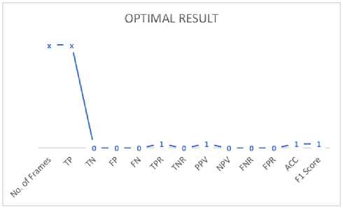
Fig.7. Optimal result graph.

Fig.7 shows an optimal result graph that has to be obtained by testing videos against performance metrics. Fig.8 shows the graphs of performance metrics for 15 different video sequences, the graphs are generated from the data of Table 1 (proposed algorithm). We can observe that except for Fig.8(n), all other results are same i.e. the values of video sequences matches exactly with the FP value of the optimal result graph shown in Fig.7.

Table 9 tabulates the time taken by all 15 video sequences which are tested under all the algorithms being discussed in this section.

Fig.10 shows the graphs of different algorithms tested agianst 15 video sequences taken in this paper for the

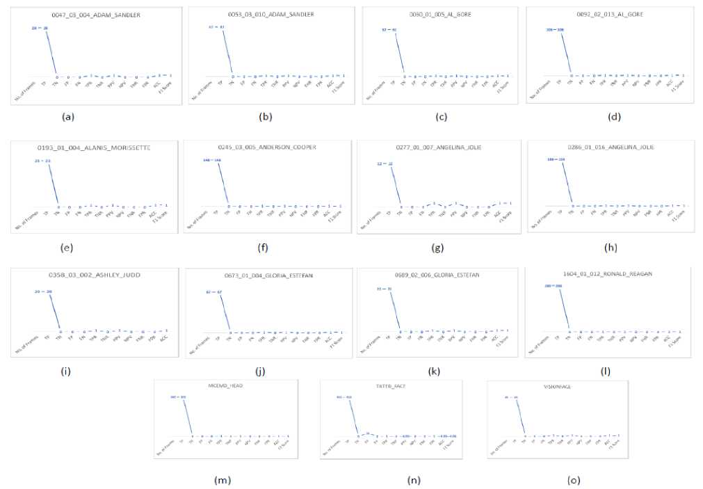
Fig.8. The graphs of performance metrics against 15 different video sequences.

Table 9. Time (sec) taken to run different video sequences by various algorithms.

VIDEO	Current Algorithm	Algorithm*	Algorithm#	KLT	CAMSHIFT	Algorithm^
0047_03_004_adam_sandler.avi	6.8	1.7	-1	-1	-1	-1
0053_03_010_adam_sandler.avi	5.6	8.3	5	5.6	-1	-1
0060_01_005_al_gore.avi	6.2	2.7	-1	-1	-1	-1
0092_02_013_al_gore.avi	6.8	3	-1	-1	4.1	3
0193_01_004_alanis_morissette.avi	6.1	2.9	3.1	5	3.6	-1
0245_03_005_anderson_cooper.avi	9.9	49.5	-1	-1	3.7	3.8
0277_01_007_angelina_jolie.avi	5.8	5	4.1	2.9	-1	1.5
0286_01_016_angelina_jolie.avi	8.5	10.9	9.8	11.7	-1	1.8
0358_03_002_ashley_judd.avi	6.3	4.6	3.3	4.7	4	1.7
0673_01_004_gloria_estefan.avi	6.2	2.7	-1	2.4	-1	-1
0689_02_006_gloria_estefan.avi	6.4	7.5	4	4.4	-1	-1
1604_01_012_ronald_reagan.avi	10.1	6	13.6	15.8	-1	-1
mcem0_head.mpg	25.7	80.6	18.9	20.4	5.8	-1
tilted_face.avi	41.4	112.8	31.4	34.6	15.5	-1
visionface.avi	10.9	15.8	6.9	8.1	5	1.3

Note: Here in Table 9 we have considered ‘-’ (fail/false condition) as -1 to plot the graphical results of the data.

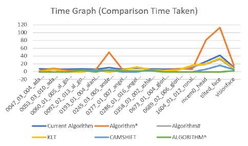
Fig.9. Cumulative time graph.

Список литературы Image training, corner and FAST features based algorithm for face tracking in low resolution different background challenging video sequences

Ranganatha S and Y P Gowramma, “Development of Robust Multiple Face Tracking Algorithm and Novel Performance Evaluation Metrics for Different Background Video Sequences”, International Journal of Intelligent Systems and Applications (IJISA), in press.
Alireza Tofighi, Nima Khairdoost, S. Amirhassan Monadjemi, and Kamal Jamshidi, “A Robust Face Recognition System in Image and Video”, International Journal of Image, Graphics and Signal Processing (IJIGSP), vol.6, no.8, pp.1-11, July 2014. DOI: 10.5815/ijigsp.2014.08.01
E. Rosten and T. Drummond, “Fusing Points and Lines for High Performance Tracking”, in Proc. of IEEE International Conference on Computer Vision (ICCV), vol.2, pp.1508-1515, October 2005. DOI: 10.1109/ICCV.2005.104
C. Harris and M. Stephens, “A Combined Corner and Edge Detector”, in Proc. of 4th Alvey Vision Conference, Manchester, UK, pp.147-151, 1988.
P. Viola and M. Jones, “Rapid Object Detection Using a Boosted Cascade of Simple Features”, in Proc. of IEEE Computer Society Conference on Computer Vision and Pattern Recognition (CVPR), Kauai, USA, vol.1, pp.511-518, December 2001. DOI: 10.1109/CVPR.2001.990517
P. Viola and M. Jones, “Robust Real-Time Face Detection”, International Journal of Computer Vision (IJCV), vol.57, pp.137-154, 2004.
http://www.mathworks.com/help/vision/ug/train-a-cascade-object-detector.html.
Elena Alionte and Corneliu Lazar, “A Practical Implementation of Face Detection by Using Matlab Cascade Object Detector”, in Proc. of IEEE International Conference on System Theory, Control and Computing (ICSTCC), pp.785-790, October 2015. DOI: 10.1109/ICSTCC.2015.7321390
Deepa and K Jyothi, “A Robust and Efficient Pre Processing Techniques for Stereo Images”, in Proc. of IEEE International Conference on Electrical, Electronics, Communication, Computer, and Optimization Techniques (ICEECCOT), pp.89-92, December 2017. DOI: 10.1109/ICEECCOT.2017.8284645
Mahesh and Subramanyam M. V, “Feature Based Image Mosaic Using Steerable Filters and Harris Corner Detector”, International Journal of Image, Graphics and Signal Processing (IJIGSP), vol.5, no.6, pp.9-15, May 2013. DOI: 10.5815/ijigsp.2013.06.02
Bruce D. Lucas and Takeo Kanade, “An Iterative Image Registration Technique with an Application to Stereo Vision”, in Proc. of International Joint Conference on Artificial Intelligence, vol.2, pp.674-679, August 1981.
Carlo Tomasi and Takeo Kanade, “Detection and Tracking of Point Features”, Carnegie Mellon University Technical Report CMU-CS-91-132, April 1991.
Jianbo Shi and Carlo Tomasi, “Good Features to Track”, in Proc. of IEEE Conference on Computer Vision and Pattern Recognition (CVPR), pp.593- 600, June 1994. DOI: 10.1109/CVPR.1994.323794
G. Bradski, “Computer Vision Face Tracking for Use in a Perceptual User Interface”, Intel Technology Journal, pp.12-21, 1998.
K. Fukunaga and L. D. Hostetler, “The Estimation of the Gradient of a Density Function, with Applications in Pattern Recognition”, in IEEE Trans. on Information Theory, vol.21, no.1, pp.32-40, January 1975. DOI: 10.1109/TIT.1975.1055330
Ranganatha S and Y P Gowramma, “A Novel Fused Algorithm for Human Face Tracking in Video Sequences”, in Proc. of IEEE International Conference on Computation System and Information Technology for Sustainable Solutions (CSITSS), pp.1-6, October 2016. DOI: 10.1109/CSITSS.2016.7779430
Ranganatha S and Y P Gowramma, “An Integrated Robust Approach for Fast Face Tracking in Noisy Real-World Videos with Visual Constraints”, in Proc. of IEEE International Conference on Advances in Computing, Communications and Informatics (ICACCI), pp.772-776, September 2017. DOI: 10.1109/ICACCI.2017.8125935
J. Strom, T. Jebara, S. Basu, and A. Pentland, “Real Time Tracking and Modeling of Faces: An EKF-based Analysis by Synthesis Approach”, in Proc. of IEEE International Workshop on Modelling People (MPeople), pp.55-61, September 1999. DOI: 10.1109/PEOPLE.1999.798346
Douglas Decarlo and Dimitris N. Metaxas, “Optical Flow Constraints on Deformable Models with Applications to Face Tracking”, International Journal of Computer Vision (IJCV), vol.38, no.2, pp.99-127, July 2000.
Dr. Ravi Kumar Jatoh, Sanjana Gopisetty, and Moiz Hussain, “Performance Analysis of Alpha Beta Filter, Kalman Filter and Meanshift for Object Tracking in Video Sequences”, International Journal of Image, Graphics and Signal Processing (IJIGSP), vol.7, no.3, pp.24-30, February 2015. DOI: 10.5815/ijigsp.2015.03.04
Stefan Leutenegger, Margarita Chli, and Roland Y. Siegwart, “BRISK: Binary Robust Invariant Scalable Keypoints”, in Proc. of IEEE International Conference on Computer Vision (ICCV), pp.2548-2555, November 2011. DOI: 10.1109/ICCV.2011.6126542
Anelia Angelova, Yaser Abu-Mostafa, and Pietro Perona, “Pruning Training Sets for Learning of Object Categories”, in Proc. of IEEE Computer Society Conference on Computer Vision and Pattern Recognition (CVPR), vol.1, pp.494-501, June 2005. DOI: 10.1109/CVPR.2005.283
D. Hond and L. Spacek, “Distinctive Descriptions for Face Processing”, in Proc. of 8th British Machine Vision Conference (BMVC), Colchester, England, vol.1, pp.320-329, September 1997.
F. S. Samaria and A. C. Harter, “Parameterisation of a Stochastic Model for Human Face Identification”, in Proc. of IEEE Workshop on Applications of Computer Vision, Sarasota, USA, pp.138-142, December 1994. DOI: 10.1109/ACV.1994.341300
“Face Database from Robotics Lab of National Cheng Kung University, Taiwan”, URL: http://robotics.csie.ncku.edu.tw/Databases/FaceDetect_PoseEstimate.htm.
Kuang-Chih Lee, J. Ho, and D. J. Kriegman, “Acquiring Linear Subspaces for Face Recognition Under Variable Lighting”, in IEEE Trans. on Pattern Analysis and Machine Intelligence (PAMI), vol.27, no.5, pp.684-698, March 2005. DOI: 10.1109/TPAMI.2005.92
A. S. Georghiades, P. N. Belhumeur, and D. J. Kriegman, “From Few to Many: Illumination Cone Models for Face Recognition Under Variable Lighting and Pose”, in IEEE Trans. on Pattern Analysis and Machine Intelligence (PAMI), vol.23, no.6, pp.643-660, June 2001. DOI: 10.1109/34.927464
Li Fei-Fei, R. Fergus, and P. Perona, “Learning Generative Visual Models from Few Training Examples: An Incremental Bayesian Approach Tested on 101 Object Categories”, in Proc. of IEEE Computer Society Conference on Computer Vision and Pattern Recognition Workshop (CVPRW), July 2004. DOI: 10.1109/CVPR.2004.383
Li Fei-Fei, R. Fergus, and P. Perona, “One-Shot Learning of Object Categories”, in IEEE Trans. on Pattern Analysis and Machine Intelligence (PAMI), vol.28, no.4, pp.594-611, April 2006. DOI: 10.1109/TPAMI.2006.79
G. Griffin, A. Holub, and P.Perona, “Caltech-256 Object Category Dataset”, Technical Report 7694, California Institute of Technology, pp.1-20, 2007. URL: http://authors.library.caltech.edu/7694
M. Kim, S. Kumar, V. Pavlovic, and H. Rowley, “Face Tracking and Recognition with Visual Constraints in Real-World Videos”, in Proc. of IEEE Conference on Computer Vision and Pattern Recognition (CVPR), pp.1-8, June 2008. DOI: 10.1109/CVPR.2008.4587572
C. Sanderson and B.C. Lovell, “Multi-Region Probabilistic Histograms for Robust and Scalable Identity Inference”, in Proc. of International Conference on Biometrics, Lecture Notes in Computer Science (LNCS), vol.5558, pp.199-208, 2009.
https://in.mathworks.com/downloads/R2018a/toolbox/vision/visiondata.
D. M. W. Powers, “Evaluation: From Precision, Recall and F-Measure to ROC, Informedness, Markedness & Correlation”, Journal of Machine Learning Technologies (JMLT), vol.2, no.1, pp.37-63, 2011.
T. Fawcett, “An Introduction to ROC Analysis”, Pattern Recognition Letters, vol.27, no.8, pp.861-874, June 2006. DOI: 10.1016/j.patrec.2005.10.010
Ranganatha S and Dr. Y P Gowramma, “Face Recognition Techniques: A Survey”, International Journal for Research in Applied Science and Engineering Technology (IJRASET), ISSN: 2321-9653, vol.3, no.4, pp.630-635, April 2015.

Еще

Статья научная