Impact of magnetohydrodynamic and bubbles driving forces on the alumina concentration in the bath of an Hall-Heroult cell

The aluminum industry is continuously increasing the productivity of electrolysis cells by increasing the line current. In order to keep an acceptable anode current density, the anode length is almost systematically increased. As a result the central channel (distance between the anodes in the center of the cell) and the side channels (distance between the anodes to the side lining) are reduced. The channel geometry, Lorentz force fields and bubbles have an important impact on the bath velocity field. We will see that the velocity field plays a key role on the alumina distribution. In order to keep an acceptable energy input when increasing the current, the anode to cathode distance (ACD) is reduced as much as possible before reaching the Magneto-Hydrodynamic constraints. This means a further bath volume reduction. The increase of current imposes an increase of alumina feeding rate simultaneously with a reduction of bath volume. Therefore, the question of dissolution, diffusion and alumina transport becomes an important element for avoiding underfeeding leading to an increase of anode effects (AE) frequency. Alumina dissolution is a very complex phenomena in which the bath chemical composition, bath temperature, alumina temperature and alumina properties play an important role [1, 2, 3]. In this

paper we assume that the dissolution is instantaneous when the alumina reaches the bath surface and concentrate the study on the diffusion and transport processes. The purpose of the study is to optimize the feeding quantities (feeding frequency), alumina feeders location and the number of feeders to minimize the number of AE and avoid sludge.

Bath velocity field in presence of bubbles and Lorentz force field: Theory

When the number of bubbles produced, per m ² and per second, is too large, a numerical approach describing the motion of each bubble separately should be disregarded.

There are essentially two standard ways to overcome this difficulty. The first consists in performing some kind of averaging over the equations and over the corresponding fields. The second bypasses the averaging and directly postulates the flow equations for each phase.

One of the main difficulties encountered when performing an averaging process is related to the possible jumps that fields can suffer at the boundaries between the two phases. One way to overcome this problem, see for example [4], consists in extending the domain of definition of each motion equation to the domain occupied by the two phases. This is achieved by multiplying each equation by the characteristic function corresponding to its domain of definition. Derivatives are then performed in the sense of distributions allowing to keep track of these discontinuities in the averaging process.

Whatever choice we make, the resulting equations will contain terms which reflect the interaction between the two phases. The exact shape of these terms are not known; they have to be defined through constitutive equations.

Motion equations

Let Ω _l and Ω _g be the domains containing the fluid and the gas respectively, with corresponding characteristic functions χ l and χ g = 1 – χ l . χ l satisfies (see [4]),

∂t χl + v · ∇χl = 0,(1)

where v is the velocity field. <  f > being the average of an arbitrary field f , we set

a(lor g) = , «(lorg) vllorg) = , and draw from (1) the averaging equation

51 a I or g)+ div («(I or g) ~i I or g J = 0.

1 (1

Let pl, pg, T, j, g, B and M i j = —I B BJ — B^lj I be respectively the fluid and gas densities, the Ц01       2

stress tensor, the electric current density, the gravitation force density, the magnetic induction and Maxwell tensor. Multiplying the MHD equations by the characteristic functions χ _l and χ _g and following the derivation used for (3) we get for the fluid and gas motions the equations

(atat~1 + < V .(V1 ® V1 ))> = v(a 1 (T + Л~i))+ piaig-<(Tl + Mt) • V/1 >,(4)

P g ( d t a g ~ g + (v g ® vg))> = v-(a gTg )+p ,g - TgVxg >, where, for anyf a „or,, f„„, = g, f >.

Approximations and modeling

In order to have a tractable model we make the following assumptions.

p2 = 0; the Reynolds tensor is included in the viscous term (a,~,) with a change of the viscous 2                                                                    ll constant which then becomes a diffusivity, (the notation will not be changed); we assume that (in Tl, Tg, T and T) p, = ~ = pg = ~g.

In order to handle the averaging appearing in the equations we consider the different terms separately (without the indices). We also assume that Maxwell tensor is not affected by the averaging process. Setting v = ~ + w, so that < x w> = 0, one gets

~~

X l                 ll where alTR = -< xlw 8 w >. Setting T = (-pI + nT(v)), where t(v) = Vv + (Vv)t we finally note that

 = = a ipI + na i T(~)-

Taking these approximations into account the equations (4) and (5) become ~ pi (51 (ai vi ) + V- (ai ~i 8 V| )) = -aiV~i + V • (ai ~) + ai V • M, +piaig —

• — i •Vxi >,

  -a V~ +V-a ~= <.W >

g g       gg g g ^.

Neglecting the surface tension effect and handling the jump conditions between the two phases in the setting used for the equations we get

~, - v1 - ~ s, and <\xi-x g )-7z 1 >-0, where ~vslip is a new field which takes into account for the averaging on the jump conditions.

Second approximation

We now make the following assumptions

V-(a g ~2)-O.(12)

and diu (av.)- 0

We moreover introduce the new field fint defined by fntt =  = .

With this assumption (10) becomes

— a gWp 2 + fM = 0.                                                  (15)

From (3) and (13) one draws

diuv1- 0                                                                            (16) 8 1 a g + diu ( a g ~ g ) -0.                                                           (17)

Constitutive equations

We will now make the assumption that the field (14), i.e. f int , is a function of ^~ v _slip only.

Following [5] we assume that

f'nt, = ^ag ~slip ,                                                                                         (18) where X is a constant. Introducing this expression into (15) yields, since by assumption ~1 = ~2,

so that

-a g V~ i =Xa g v sii P .                                                              (19) ~ v slip ~-^ "                                                            (20)

The coefficient λ has to be determined experimentally.

The model

With the above results we are now ready to give the equations on which our model is leaning.

Fluid averaged equations pi(dt(ai~i) + V - (ai~i 8 ~i)) = -V~ + V - (a,~)+a,V- Т~, + p,aig.

Gas averaged equations

51 ag + diu (ag ~2 ) = 0, aV~1 +aXv6= 0

Jump averaged conditions

~2 = ~1 + ~ slip, ai + ag = 1.

Boundary conditions on the different fields have to be added.

Alumina diffusion and convection: Theory

Let Ω ⊂ R ³ be the domain representing the cell, Ω b be the bath, and Ω a the anodes.

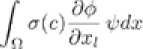
Current density

The current density distribution in the bath is a function of alumina concentration, and is given by where is the potential, and σ is the electrical conductivity, which depends on the alumina concentration c.

Since diυ j = 0, we get with following the boundary conditions (jǀn) = j0 on the anodic rod,      on the bath-metal interface, d ■           1 h

.

The current j = ( j ₁; j ₂; j ₃) is then computed in the following way to avoid rough approximations.

/ ji ydx = - for suitable functions , and l = 1; 2; 3.

The model will take into account the analysis of the parameter σ as a function of the bath composition.

Alumina distribution

In this study, it is assumed that the alumina feeding is known, and that the dissolution is instantaneous. The alumina distribution in the bath Ω _b is given by the following partial differential equation

• - ^di^u ( a ( x , t )) V с ⁽ x , t ) + ^{(v (} x , t ^)v с ⁽ x , t ) ) = 0,                                             ⁽ 3 ⁰⁾

where

• –    c is the alumina concentration in mol/m³,

• –    α is the anisotropic diffusion coefficient. A value of 0,5 m²/s was determining the Reynolds mean tensor. It also leads to an average alumina concentration reflecting industrial cells.

• –    v is the velocity field in Ω _b induced by the bubble motion, and the MHD.

The boundary and initial conditions have the following form.

• –    The concentration c is given on the feeder.

• -    The concentration flux on the anode and the bath-aluminum interface is a — + p ( jn ) = 0; the coe 8 n

cient в verify P =    if [ c ] = mol/m , with z is the valence, and F is the Faraday constant, in our case z = 6.

zF dс

• -    a— = 0 elsewhere,

8 n

– c is given at time t = 0.

Weak formulation

Let us use the following notations.

• –    Г _b is the bottom of the cell (the metal-bath interface),

• –    Г a is the top of the anodic rod (the entrance of the current),

• –    Г f is the feeder domain,

• –    Г ab is the interface between the anode and the bath.

With these notations, set equipped with the norm equipped with the norm

The weak formulation of problem (28) is:

Find such that,

Then the computation of the current density j = ( j ₁; j ₂; j ₃) is obtained from equation (29)

. •*.>.■•:. Finally, the weak formulation for the alumina concentration is: Find с e L ( 0, T;H ’( Q b )) with c = c f on F f , such that

• ,                  X           г                           г

Jq^ \Ut          /       Jgb                    •'Г^иГь

Numerica met o s

Let us decompose the domains Ω, and Ω into classical tetrahedral finite element mesh. For the

b numerical simulations of problems (33), (29), and (34), the following algorithm is used.

– Initialization

An initial alumina concentration distribution c ₀is given at time t = 0. Let τ be the time step.

– Iterations

m

For time t_m = m ∙ τ , if c _h is the concentration at time t_m

• a)    Compute the electrical conductivity c = c ( c ” ^.

• b)    Find         such that,

• c)    The electric current j h = ( j h ;1; j h ;2; j h ;3) is obtained as, ∀ l = 1; 2; 3, and

• d)    A BDF scheme of order 2 [6] is used for the time discretization of the concentration equation (34). Moreover a Petrov-Galerkin streamline diffusion method is applied for the advection term [7, 8]. We get the following equation ( 5 small parameter).

Find c ” ^{+ 1}, solution of

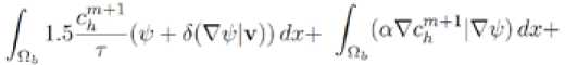
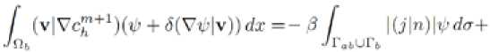
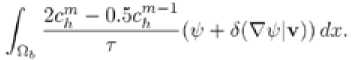
for all

Alumina diffusion and convection:Industrial cell

In this section some numerical result for the computation of the alumina distribution in the bath are presented. On the feeders, the alumina concentration is set to 5 % of the bath weight. As a stationary solution is presented, continuous feeding is assumed. The impact of dump feeding could easily be analysed.

Figure 1 correspond to the stationary alumina distribution, when the velocity is neglected. The concentration is shown under the anodes. The two feeders locations appear clearly in the figure. The asymmetry of the diffusion pattern reflects the larger channel width at the feeders. Figure 2 shows the alumina concentration under the same conditions at metalbath interface level. Away from the feeders, at a distance larger than about one anode width, the concentration is close to 2,55 %. The vertical variation of the alumina concentration is 0:5 % under the feeders. It is negligible away from the feeders.

In fig. 3, the velocity streamlines induced by the MHD are presented.

The impact of this velocity field is shown in fig. 4.

The previous cases did not take the bubbles into account. It is well known that they have an important effect on the velocity field. Moreover the considered cell has slotted anodes. This also has an

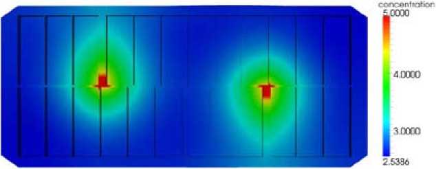
Fig. 1. Alumina concentration in the bath when the velocity is zero, under the anodes

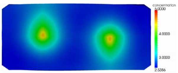
Fig. 2. Alumina concentration in the bath when the velocity is zero, bath-metal interface

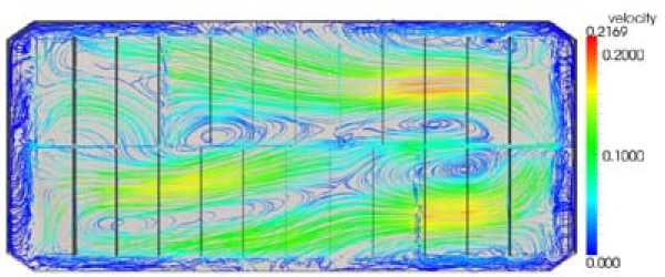
Fig. 3. MHD velocity in the bath (streamlines)

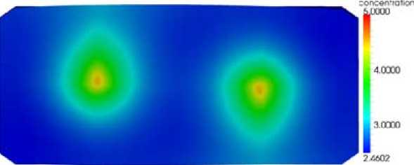
Fig. 4. Alumina concentration in the bath when the velocity is induced by the MHD

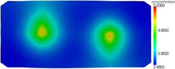
Fig. 5. Alumina concentration in the bath, velocity induced by MHD, bubbles, and slots

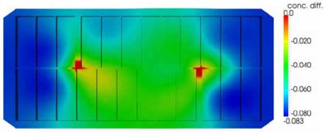
Fig. 6. Alumina concentration variation due to MHD [ %]

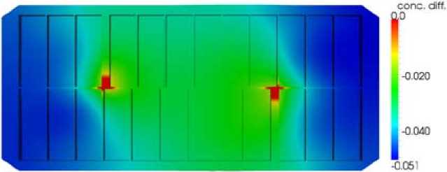
Fig. 7. Alumina concentration variation due to MHD, bubbles, and slots [ %]

impact on the velocity. Figure 5 considers the case when the velocity field consists of the effects of the MDH, the bubbles, and the slots in the anodes.

From the different figures, the alumina concentration field appears as slightly modified by the velocity field. However, when considering the concentration evolution, the time needed for reaching the stationary state is reduced by a factor 2 in any situation when the velocity field is acting. Therefore the velocity field plays an important role in the feeding process (alumina dumps).

To highlight the role of the velocity field, fig. 6 and 7 show the difference between the alumina concentration field due to the diffusion only and in presence of MHD velocity, resp. total velocity field.

The highest diааerences are observed at the ends of the cell, due essentially to the MHD effects. High negative values relate to high alumina concentration difference. The effect of bubbles and slots generate turbulence, homogenizing the concentration distribution.

Conclusions

A new model for the velocity field in presence of MHD, and small bubbles is developed. This velocity field is used to determine the evolution of the alumina concentration using a non-stationary convection-diffusion equation. This equation takes into account the feeding, and the Faraday law at the anodes and cathode.

The application to an existing cell with two point feeders demonstrate the following:

• –    The alumina concentration can vary up to 2,5 %. Typically a variation 1 % can be expected between anodes.

• –    The time needed to reach the stationary state due to the diffusion process only is twice the one for the case with MHD and bubbles effects velocity fields. It was found around two minutes.

• –    The velocity field has an important effect for the alumina distribution under the anodes. It helps to homogenize the alumina concentration.

• –    Bubbles and slots modify the velocity field which generate turbulences leading to increased homogenizing effects.