Impact of Model Mobility in Ad Hoc Routing Protocols

Published Online September 2012 in MECS

I ． INTRODUCTION

Computer science has continued to evolve in recent years in various areas, particularly in the field of communication. Indeed, the limits of the communication between the men were extended dramatically thanks to computer networks. Since their emergence, the networks have become increasingly fast and powerful. The first links in this evolution are the wired networks, which are bulky and rigid. The networks have then earned in freedom with the emergence of the wireless technology, offering more flexibility, more speed and less expense. Then, computer networks have entered the era of mobility. New technologies have emerged, allowing the units of the network to move freely while being connected together. With the proliferation of lightweight devices (PDAs, laptops, mobile phones), mobile communication networks have become more efficient and accessible, and push researchers today to try to achieve the goal of networks: "Access to information anywhere and anytime".

In this paper, we will study the impact and the effect of node mobility in wireless Ad Hoc network using deferent models of mobility and diverse routing protocols implemented in GloMosim simulator presented in the coming sections, a mobile Ad Hoc network is a self-organizing network formed spontaneously from a set of communicating mobile entities (laptops, mobile phones, PDAs) without the need for pre-existing fixed infrastructure [1]. Other proposed names for this type of network as being infrastructure less wireless networks, instant infrastructure [2] and mobile-mesh networking [3].

The rest of this paper is organized as follows. Section 2 and 3 first describe the routing process in ad hoc network and the mobility models existing in those networks. Section 4 describes the Random Waypoint model and section 5 presents the Gauss markov model for mobility. Section 6 presents the algorithm to be implemented in GlomoSim. Section 7 and discuses the results collected from the environment of simulation. Finally, Section 8 concludes the paper.

• II.    ROUTING IN AD HOC NETWORK

One of the major technological challenges of such networks is that they require new types of routing protocols. As opposed to the wired infrastructure, there are no dedicated router nodes: the task of routing needs to be performed by the user nodes, which can be mobile, unreliable and have limited energy and other resources.

Ad hoc routing protocols have been classified into on-demand and table-driven protocols. Between these two, many hybrid approaches have been developed. The increasing size of the ad hoc networks considered made necessary the use of techniques such as geographical routing and hierarchical routing [3]. Finally, in many deployments of ad hoc networks, the problem of energy conservation takes precedence from all the other performance metrics, thus power aware routing protocols will be treated in the futures papers. In this paper we will focus on two major routing protocols: AODV and WRP, to see the effects of mobility models.

The AODV (Ad hoc on-demand distance vector) routing protocol was developed by Perkins and Royer as an improvement to the Destination-Sequenced Distance-Vector (DSDV) routing algorithm [4]. AODV aims to reduce the number of broadcast messages forwarded throughout the network by discovering routes on-demand instead of keeping complete up-to-date route information.

WRP (Wireless routing protocol) [5]: Murthy and Garcia propose WRP which builds upon the distributed Bellman-Ford algorithm. The routing table contains an entry for each destination with the next hop and a cost metric. The route is chosen by selecting a neighbor node that would minimize the path cost. Link costs are also defined and maintained in a separate table and various techniques are available to determine these link costs.

Most of works in literature regarding simulation routing protocol, take in consideration only one model (random waypoint model), the goal of this paper is to show that the mobility models can affects considerably the performances of routing in the wireless network. For all the reasons cited we will improve one of the very used models of mobility (Gauss Markov), by treating all cases of mobility (Speed, direction, borders detection)

• III.    THE MOBILITY MODEL

The mobility model is designed to describe the movement pattern of nodes, and how their speeds and directions are changed over the time. Currently there are two types of mobility models used in the simulation study of M\ANET: traces base model and synthetic base model [6].

The traces base model obtains deterministic data from the real system. This mobility model is still in its early stage of research, therefore it is not recommended to be used. Choosing suitable movement pattern depends on applications that use the model.

The synthetic base model is the imaginative model that uses statistics. In the real world, nodes or objects have their target destination before they decide to move. However, the movement of each mobile node to its destination has a pattern that can be described by a statistical model that expresses the movement behavior in the real environment.

A mobility model defines the movements of mobile nodes during a simulation of a mobile wireless network in a given area. These models can define free movements or restricted by mobility constraints (speed limit, presence of obstacles) [7].

Several models are defined in the literature to simulate the behavior of nodes. These models are divided into two classes according to the method of moving nodes. In the first class (mobility models by entity), the nodes move independently of each other (these models can be classified according to the randomness of their movement, either a movement is completely random with no memory of the past, or a movement is flexible where changes in speed, direction and position at every moment are based on the previous state.). While in the second class (mobility models by group), the nodes move in groups [7].

This type of mobility model can be either Entity Mobility Model (EMM) or Group Mobility Model (GMM). In EMM, each node moves independently. Examples of this type of mobility model are Random Walk [8], Random Waypoint [9] [10], and Gauss Markov [11]. For GMM, the movement of each MN depends on some other MNs in the group. The major problems of using this model are shape turn and sudden stop.

In our study we used Random Waypoint mobility model as it has been widely used in the simulation study of MANET, despite some unrealistic behaviors such as sudden stops and sharp turns. While the mobility model of Gauss-Markov has shown that it can solve both problems. So we added this model to see the impact of different mobility models on the performance of protocols.

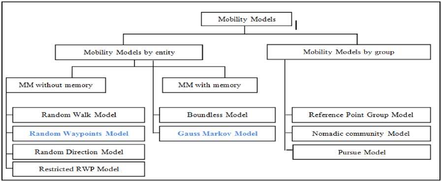
Figure 1: The class of mobility models.

• IV.    RANDOM WAYPOINT MODEL

  This model is the most used in experimentations and simulations. One reason for its popularity it’s the presence in the most popular simulators [15]. This model was introduced by Johnson and Maltz in 1996 to study the performance of DSR (Dynamic Source Routing) routing protocol. This model incorporates movement phases and phases of break: At the beginning of its movement, a mobile node selects a destination

from the area of simulation: it chooses two x and y coordinates according to a uniform distribution on the interval [0, xMax] and [0, yMax] (where xMax and yMax are respectively the length and the width of the simulation area). It then chooses a uniformly value for speed in an interval [min speed, max speed]. Once the movement is completed, it enters a phase of pause of some duration. The parameters of this model are the minimum speed, maximum speed and pause time [2].

It was found that the spatial distribution of nodes is concentrated in the middle of the area after a simulation run time. Note that the Random Waypoint is close to the Random Walk with the difference that the selected destination is always a point inside the simulation area, eliminating any edge effect. Fig 2 has illustrated the displacement of a node using the Random Waypoint.

Absolutely random effect is obtained by placing alpha = 0 and a linear effect is obtained by placing alpha = 1. To ensure that a node does not stay near one edge of the simulation area, nodes are pushed away the edge when they are within a certain distance from the edge. Fig 3 shows the displacement of a node using the Gauss Markov model that we implemented in C + +.

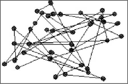
Figure 2: Displacement of a node using the Random Waypoint [10].

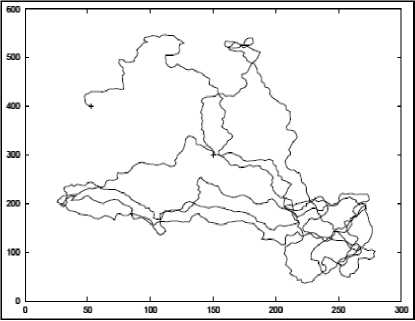
Figure 3: Displacement of a node using Gauss Markov Model.

• V.    GAUSS MARKOV (GM)

This model was used for the simulation of a protocol for ad hoc networks. Gauss Markov mobility model is similar to the Boundless, in the sense that the position and velocity at any time, depend on the position and velocity of the previous moment [8]. Speed, direction and position of a node vary according to the following formulas:

Sn = Sn-1 * alpha + (1 - alpha) * S

+sqrt (1-alpha 2) * SXn-1;                (1)

Dn = Dn-1 * alpha + (1 - alpha) + D

* sqrt (1-alpha 2) * DXn-1;               (2)

Where the parameters Sn, Dn, alpha, S, Sxn-1, DXn-1, are defined:

S N : Speed at time n.

D N : Direction at time n.

ALPHA : Parameter between [0,1], used to vary the randomness of the movement.

S : fixed value that represents the average speed when n > ∞.

• D : Fixed value that represents the average direction When n > ∞.

Sxn-1 , Dxn-1 : Random variables from a Gaussian distribution.

Specifically, at time n, a position of mobile node is given by the equations:

Xn = Xn-1 * + Sn-1 Cos (Dn-1);          (3)

Yn = Yn-1 + Sn-1 * Sin (Dn-1);           (4)

In GloMosim Gauss Markov is not implemented so, our first contribution is to implement the Gauss Markov model in GloMosim 2.3[15] simulator. And after that we study the performance of routing protocol by making comparison between WP models. The algorithm of GM is presented in the section bellow.

• VI. ALGORITHM OF GAUSS MARKOV (GM)

The algorithm of GM is presented as described in the following algorithm:

Begin

01: Variables:

01 nb_nodes, bound_x, bound_y, tm_sim: int;

03: Alpha, max_velocity,inean_velocity, mean_direction, y_tmp, x, y: real;

04: Treatments

05: Fornb = 1 to nbnodes //scan all existing nodes

06:

07:

08:

09:

10:

11:

12:

13:

14:

15:

16:

17:

18:

19:

20:

21:

22:

23:

24:

25:

Ц Random initial Position for node x =uniforinrandomvariable (0, bound_x);

у =uniform_random_variable(D, bound_y);

// Node position in evry instant t

For t=l to tmsini

I* Calculate the new position by using the new formula of Gauss-Markov*/ x_tmp =x+velocity*cos (direction);

y_tmp =y+velocity*sin (direction);

normal_velocity =norinal_random_variable[O,1];

normal_direction=normal_random_variable [0,1];

velocity_tmp=alpha*velocity+ (l-alpha)*mean_velocity

+SQRT (1-alpha2) "normal_velocity;

direction_tmp =alpha*vct_direction+[l-alpha)*mean_direction +SQRT (l-alphaz) *normal_direction;

//Boreders traitement

77x_tmp< dist bord Then mean direction =0;

7fx_tmp> bound_x-dist_bord Then mean_direction =180;

77y_tmp< dist bord ТЛел mean direction =90;

End

26: END

END;

Figure 4: Gauss Markov Algorithm.

Where parameters are defined:

• •    nb_nodes: number of nodes.

• •    bound_x, bound_y: Simulation dimension.

• •    tm_sim: time of simulation.

• •    Alpha: random degree.

• •    max_velocity: maximum speed.

• •    x, y: positions of nodes.

Initially, the nodes are randomly distributed on the area of simulation. To calculate the new positions using the speed and direction are calculated in the previous moment, they initially are randomly distributed respectively on (0 ... maximum speed) and (0 ... 360 °). According to the above formula for the coordinates exceed the limit of the zone, so to ensure that a node does not stay near one edge of the simulation, nodes are pushed away from the edge when they are less some distance from the edge (we chose 10m). This effect is achieved by modifying the value of the average direction mean_direction during the simulation. When a node is near the right edge, the value of mean_direction changed 180o. If it is near the left edge, the value of 0o mean_direction changed. If it is near the lower edge, the value of 90o mean_direction changed, and if it is near the top edge, the value of mean_direction changed 270o, as is illustrated in fig 6.

After implementing this algorithm using C++ language we find the following results, we can find also many scenarios by changing the value of alpha:

• When α=0 the node are very instable.

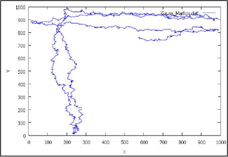
Figure 5: absolutely random (α=0).

• When α= 0, 75 and there is no treatments of borders we will have the following situation.

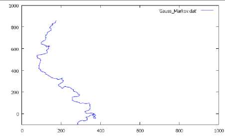
Figure 6: Without avoiding the edges (α= 0,75).

• When α=1, the movement of node is linear.

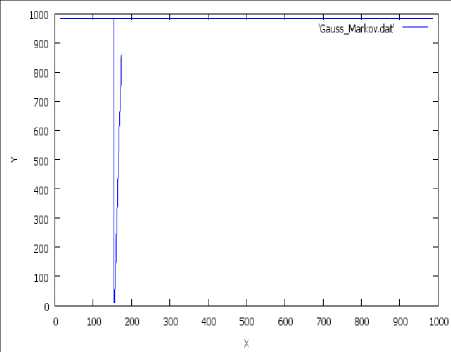
Figure 7: Node movement very linear (α=1).

• VII.    THE SIMULATION ENVIRONMENT

The simulation consists in reproducing an abstract representation of the system studied using the GloMosim simulator [11].

We implemented the proposed algorithm both with C++ and glomosim-2.03[15], it’s a library scalable simulation environment for wireless network system using the parallel discrete-event simulation capability provided by PARSEC [16] , PARSEC is specific language based on C developed at UCLA (the University of California). GloMoSim respects the OSI model and associates an object to each layer. We set their parameters as follows:

T able 1. P arameters used in simulation .

Size of the area (m x m)	1000 x 1000
Simulation time(S)	300
Bandwidth (bits/s)	2000000
Transmission range(m)	250
Type of the MAC layer	IEEE 802.11
Radio propagation model	Free space
Type of traffic	CBR
Type of Mobility model	RW|GM
Number of nodes	10|20| 30 |40|50|60
Routing protocol	WRP|AODV

T able 2. R andom W aypoint parameters .

Pause time(s)	0| 10 |100|200|300
The maximum speed (m/s)	10

T able 3. G auss M arkov

Alpha (degree of random)	0|0.25|0.5| 0.75 |1
The maximum speed (m/s)	5| 10 |50

All network nodes were located in a physical area of size 1000×1000 m² to simulate actual mobile ad hoc networks. The selected mobility model was the Random Waypoint model and Gauss Markov Model.

For random waypoint, a node randomly selects a destination from the physical terrain, and then it moves in the direction of the destination in a speed uniformly chosen between the minimum and maximum roaming speed. After it reaches its destination, the node stays there for a specified pause time period. In our simulation, the value of minimum roaming speed was set to 0m/s and maximum mobility speed was 10m/s.

The simulation time of each run lasted for 300 seconds. Each simulation result was obtained from an average of the 10 simulation statistics. The traffic generators were CBR. The generators initiated the first packet (i.e., start time) in different time and sent a 512 bytes packet each time.

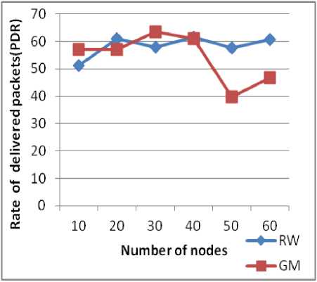
Figure 9: WRP PDR based on the number of nodes.

• VIII.    ANALYSIS AND RESULTS

Performance metrics that have been used to analyze MANET are as follows (they are applied both on AODV and WRP):

• •    Rate of delivered packets (PDR):

This is the ratio between the number of data packets received by destinations and the number of data emitted by the sources.

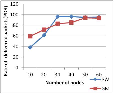
Figure 8: AODV PDR based on the number of nodes.

For AODV (Fig 8) there is parallel increase of the number of packets delivered compared with number of nodes, and from 50 nodes there is stability for both models. There is a remarkable difference between using RW and GM as a mobility model for performance evaluation protocol WRP (Fig 9) at different densities. We note that the delivery rate for both models is less than in the PDR for AODV because in proactive protocols, packets are sent before the routing tables converge to a stable state, and they are sent over broken roads that are assumed valid as opposed to reactive protocols that react to failures of links.

• •    End To End Delay in Ms (EED):

The average time taken by a packet to move from a source node to destination node.

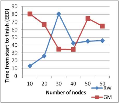
Figure 10: EED based on the number of nodes (AODV).

There is a remarkable difference between the use of RW and GM for performance evaluation of AODV protocol for different densities. In WRP there is a growth delay transfer function of the growth of the number of nodes, and if the density exceeds 30 nodes there is no relationship between the number of nodes and the transfer delay whatever the model. Note that the timeout values for both models are less than the delay seen in AODV because the proactive construct and maintain routing tables permanently. This eliminates the time of discovery of roads unlike reactive protocols.

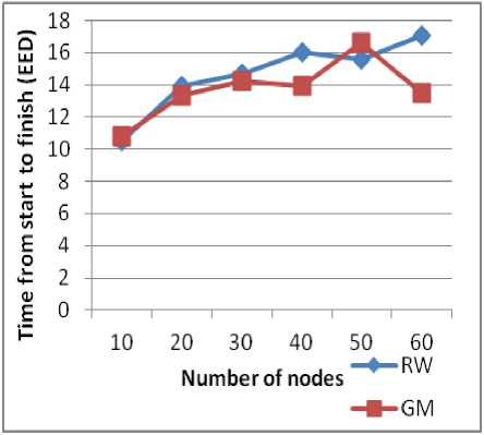
Figure 11: EED based on the number of nodes (WRP).

• •    Number of control packets (OH):

The control information provides data the network needs to deliver the user data, for example: source and destination addresses, error detection codes like checksums, and sequencing information. Typically, control information is found in packet headers .

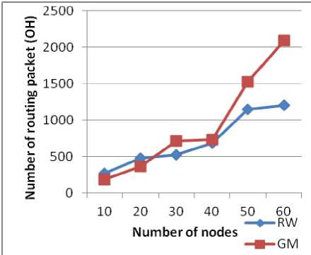
Figure 12: OH based on the number of nodes (AODV).

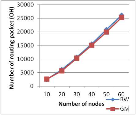
Figure 13: OH based on the number of nodes (WRP).

In AODV, we note that for a small topology the number of routing packets using RW is a bit higher than using GM. With the increasing of the number of nodes, the number of routing packets using RW stabilizes but with GM it grows. In WRP, there is a linear growth in the number of routing packets with the number of node for both models, with a small increase for the RW. Note that the values of OH for both models are very large compared to OH seen in AODV because the proactive protocols generate periodic messages while reactive protocols generate messages as needed.

Now we focus our experimentation on the variables of model GM as speed, direction and alpha in order to see the impact on the performances of AODV as example.

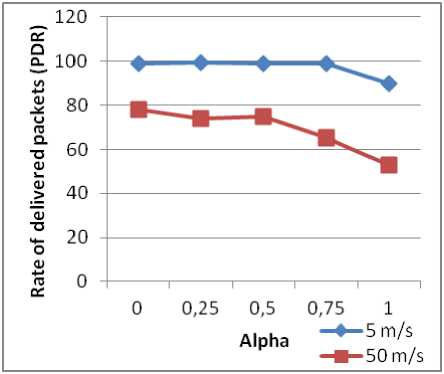
Figure 14: PDR based on alpha and maximum speed (AODV).

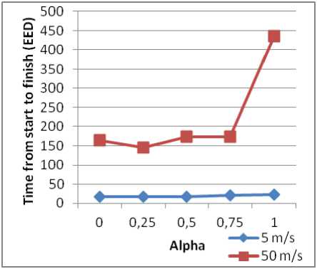
Figure 15: EED in ms based on alpha and maximum speed (AODV).

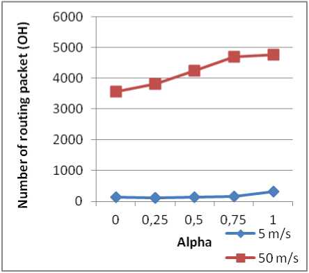
Figure 16: OH based on alpha and maximum speed.

For normal speed the rate of packets delivered is high (nearly all sent packets are received). When the speed is high, the PDR decreases for a value of alpha < 0.5 and when alpha > 0.5 there is a decrease of PDR for a normal or high speed. If speed is high, there is a remarkable difference for different values of alpha for the delay. For OH, there is a growth of the latter with the growth of alpha. If the speed is normal, delay and OH are almost stable for all values of Alpha. With increasing speed, there is an increase of OH and the same remark quoted for the transfer delay.

• IX. CONCLUSION

In this study, we implemented the mobility model Gauss Markov using C++. Then, we have integrated into the Network Simulator (GloMoSim) on which we simulated the routing protocols AODV and WRP with two mobility models RW and GM. After our simulations, we found that the performance of routing protocols vary depending on mobility models used. Also that for the same model, the choice of parameters also affects the results. So the mobility model must be considered when designing a routing protocol. This study allows us to better understand the factor of mobility in ad hoc networks. We propose in our future work to study and see the impact of mobility model on energy consumption