Implementation of gray level image transformation techniques

Published Online May 2018 in MECS DOI: 10.5815/ijmecs.2018.05.06

A description of a two dimensional light intensity function f(x,y), where the letters x and y represents spatial co-ordinates and the ‘f’ value at every point is directly relational to the gray level of the image at that point is known to be an image [1]. Digital image processing methods alters the deficiency in an image into a modified improved version. From computer science, image processing is some process of signal processing which takes on an image or frames of videos as the input and outputs either an image or set of parameters that is connected to the image [2]. Lately, image enhancement has become one of the central topics in image processing. Image enhancement includes a collection of skills that are used to improve and develop an image visual appearance - a description in Fig 1- or a conversion of the image to an improved form for suitability and understanding of human and machine interpretation.

f(x,y)^ T -> g(x, у) = т[/(х, у)]

Fig.1. image description equation

Several kinds of image and pictures are employed as the basis of information in recent communication system and broad-based applications. Most images taken may have inherit some form of degradation such as blurred image. Similarly, an image converted from certain form to another such as scanning, transmitting, storing and a lot more may also inherit some form of distortion. Mostly the degradation may occur at the output and therefore the need to enhance the output image for an improved visual appearance and appealing.

The chief goal of enhancement of an image is to process the image such that the outcome serve the purpose for which it was intended for a specific target or set application. In most situations, the end effect of image enhancement can be recognized visually. Although enhancement of image is very challenging issue in many research and application areas, this aspect of image processing is a necessity and needs expanded research to address certain technical challenges that occur in daily operation. Image enhancement techniques is needed to address or handle regular objects with regards to image geometric transformations or recover certain characteristics by adjusting the intensities or colors for the processing of medical images and other areas of application of image processing as biometric image processing, satellite image processing etc. There has not been any general theory of image enhancement partly due to the fact that no universal standard for the quality of an image has been proven. Once an image is taken for visual interpretation, the eyewitness is the definitive judge of how well a specific approach works. Thus leading to the development of varying classes of techniques over the past decades [3 and 4].

A full proof implementation of gray level image transformation is possible but a challenging task. In 2001, to automatically find a measure for central tendency of an image brightness histogram, [5] created an automatic contrast enhancement technique by shifting and converting the histogram appropriately. A contrast enhancement algorithm based on curvelet was proposed by [6] which tapped the properties of curvelet for contrast stretching for effective enhancement of image contrast. This approach is very efficient for correcting images which may contain noise. A cumulative function was put forward by [7] to be used in together with histogram equalization to realize contrast enhancements. In this paper an implementation of gray level image enhancement techniques is undertaken. A software program developed in MATLAB is used to apply the techniques studied. The next section presents the related works of the topic under discussion. The remaining of the paper is organized as follows: In section III Gray level image transformation techniques is introduced followed by section IV with a brief explanation of the application of MATLAB and its implementation of the software. Section V details the simulation experiment and results. Finally the paper concludes with Section VI.

• II.    Related Works

The main purpose of image enhancement is to enliven the quality and present an improved feature of an image that is better than the original one. In simple terms, Image enhancement techniques try to boost the quality of an image for clearer and easier human or machine interpretation resulting in higher perceptual quality of images.

Most medical imagery is presented in grayscale; tumor detection imagery is no exception. Kalaiselvi et al [8], identified a novel technique to detect Brain Tumor boundary by applying a bi-modal fuzzy histogram thresholding and edge indication map. Their technique first sharpen a gray level image and apply a generated hybrid approach to obtain desired output.

From various fields in image processing domain, a common practice is the process of generating histogram from a given gray level image. In their work, [9] presented an approximation technique for a quick generation of image histogram of grayscale images. Their approach help reduce significantly the time needed to complete a histogram generation of a gray level image and additionally presents acceptable histogram for onward processing.

Buffering has been a significant area of concern in recent times in image processing. To process and present an enhanced image, [10] presented an efficient buffering technique for reading data in to memory. Their method not limited to color, also implemented gray level images using four different optimum window size and compared their timing efficiency and area utilization.

A variant of dual mutation DE for image contrast enhancement application of was introduced by [11] to improve the details and contrast of images. Their technique aims to increase the fitness criterion which considers entropy and edge information of the image.

Again With a differential evolution optimization technique, [12] attempted to implement gray level images by demonstrating the adaptability and effectiveness for locating global best solutions to details of an image. Their technique which adopt a transformation function of parameterized intensity as an objective function resulted in achieving desired image.

Enhancing an image involves maximizing the content of image information by an intensity transformation function. [13], applied this method for enhancing graylevel images to achieve promising results by considering image enhancement as an optimization technique and applying particle swarm optimization. Similar approach for gray-level implementation was adopted by [14] on multi-resolution gray-level image.

• III.    Gray Level Image Transformation Techniques

Almost all Image processing techniques is largely focused on gray level transformation techniques as gray level transformation operate directly on pixels i.e. an image is improved by adjusting the pixel intensities directly (not as a result of certain other parameter finetuning in a varying domain). Each technique modify the pixel values according to its procedure depending on original pixel value i.e. local or point process. Ideally, a gray level image generally involves 256 levels of gray, so from the histogram, the horizontal axis spans from 0 to 255. On the other hand, the vertical axis which differs in scale is dependent on the number of pixels in the image and the gray level values distribution. The simplest of all image enhancement techniques has the formula as

s = T *r (1)

where T is a transformation that link a value of pixel, r onto a value of pixel, s and the pixels values before and after processing, will be designated by r and s , respectively. Let r = f(x,y) s = g(x,y), r and s denotes gray levels of f and g at (x,y).

Numerous techniques as discussed in the next section exist to compare the pixel values with their close or neighboring pixels with Fig 2 depicting some basic gray level techniques adopted. However which ever technique which is adopted and applied, the objective is to enhance the appearance of the image in all sense including human and machine perceptions by alternating the dominance of some characteristics, or by decreasing the uncertainty between dissimilar regions of the image.

• A.    Image Negative

This is perhaps the simplest technique in image transformation. The negative of an image has gray levels which lies in the range [0, L-1] and is obtained by using the given expression s = (L – 1) – r (2)

which therefore achieve the results in Fig 4. The workings of this technique is such that, each value of the input image is deducted from (L-1) equation and linked to the output image.

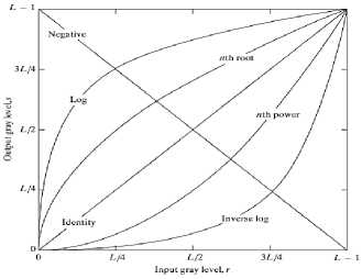
Fig.2. Some gray Level techniques

The reverse of an image intensity levels in such a manner results in the correspondent of a photographic negative. An example of this technique is shown in Figs 3 and 4

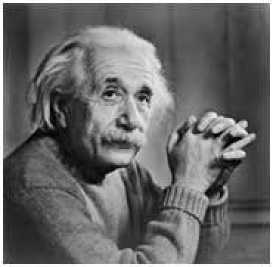
Fig.3. Original image

In an 8 bit environment (as used by Fig 3) the number of gray levels in the image are 256. When applied in the equation 2, it becomes s = 255 – r

Thus each value is subtracted by 255 resulting in lighter pixels becoming dark and the darker picture becomes light hence the image negative.

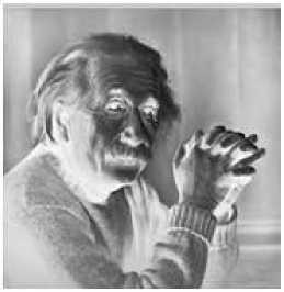
Fig.4. Image Negative

This processing technique is particularly suited for improving white or gray element embedded in dark regions of an image, particularly when the dark areas have a dominant size.

• B.    Gamma Transform

Gamma transform is also called power-law transform. i t is mathematically denoted by the following equation:

f(x,y) = c* f(x,y)Y            (4)

where the random positive constants is denoted as c and y, r is the intensity of the original image and s representing transformed images intensity with the intensity profile 0 through 255. This intensity transformation characteristic is illustrated in Fig. 5. with varied γ values. Gamma transformation with fractional γ value corresponds low intensity values to high intensity values i.e. maps slighter darker range of output to broader range of lighter output values [2].

Moreover, with this technique, the characteristic curve can be adjusted by tuning γ, and therefore can modify the slightness of darker and broadness of the lighter intensities of an input image. It can be understood from Fig 5 that, with γ = 1, identity transformation is the unit ramp characteristic that would be realized and γ > 1 and γ < 1 will have precisely an opposite effect with reference to fractional values of γ .

It is to be noted that, various display devices possess certain gamma correction algorithms, which explains why images are displayed at different intensity. This is

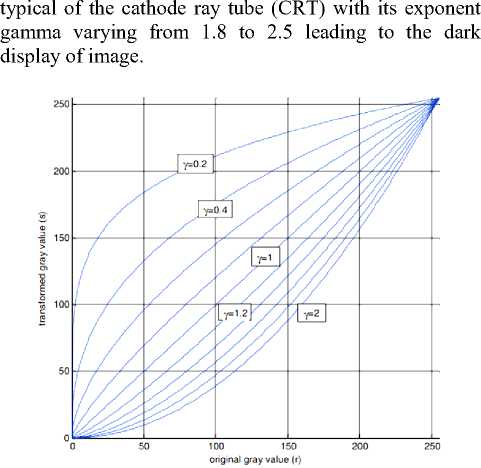
Fig.5. Transfer characteristics for power-law intensity transformation

Since gamma of different display devices are different, it is by far the most primary technique adopted to enhance images for several display devices.

A pseudo-code for Gamma correction is illustrated below

• 1.    Get image

• 2    if image is RGB convert to grayscale else continue

• 3.    Set gamma value

• 4.    Apply equation 3 to image

• 5.    Output image

• C.    Logarithmic transformations

This is consist of two type of transformation, Log transformation and inverse log transformation [1]. The conduct of inverse log transformation technique is directly opposite of the logarithmic transformation therefore any transformation characteristic curve with the same approach will perform precisely as the log transformation, i.e. expanding one part of the intensity profile and compressing the other.

The log transformations can be defined by this formula s = c log(r + 1)                   (5)

with s and r representing the values of the pixel of both output and input image and c is a constant with intensity profile spanning from 0 to 255. The value 1 from equation (5) is included to each pixel value of the input image to make the minimum value at least 1 and to eliminate a pixel intensity value of 0 in an image which will then lead to log (0) which results to infinity.

The operation of this technique is that such that, it enhance the dark pixels in an image at the expense of the higher pixel values. This therefore results in the mapping of an original input image, narrow range of lower intensity value to a wider range of output levels and a reverse mapping of a wider range of higher intensity values to a narrower range of output gray levels. This technique is mostly preferred when the image objective is to enhance dark pixel and compress brighter pixels.

With inverse logarithmic transformation also called Exponential transformation, higher gray levels intensity is extended at the expense of lower gray level intensity.

It can be defined by this formula s = exp [(r)*c - 1]                   (6)

• D.    Piecewise-Linear Contrast stretching

To increase the range of brightness values composed of by an image, this enhancement technique is used, so that the image can be analyze in an enhanced and efficient manner. The objective value of an image contrast may differ partly due to certain features such as illumination quality or setting of the acquisition sensor device. This therefore calls for the need to control the contrast of an image to do away with the difficulties in image acquisition. In simple terms, Contrast is explained as the alteration between maximum and minimum intensity of pixel in an image. The core motive behind contrast stretching is to expand the range of dynamic gray levels of an original image to result in an enhanced image process. Therefore, this approach ends in adjusting the dynamic range of the grey-levels of an image of interest. Fig 6 shows a typical transformation used for contrast stretching. The positions of points (r1, s1) and (r2, s2) manipulates the profile of the transformation. Contrast Stretch technique presents the simplest contrast stretch method that widens the values of pixel of an image with low-contrast or high contrast by spreading the dynamic range through the entire image spectrum from 0 – (L-1).

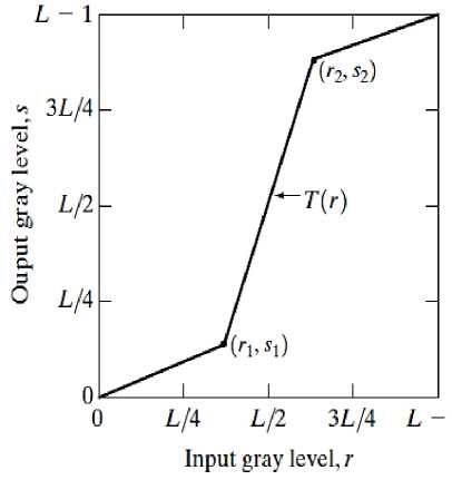
Fig.6. Contrast stretch graph

• E.    Gray Level Slicing

This technique is adopted when a specific range of gray level is gains prominence and is needed to be applied to enhance an image i.e. to suppress or maintain some details of significance. It although relatively similar to thresholding, it diverges a slightly in its operation. This technique is most preferred in analyzing most health and satellites images to obtain further analysis. It is particularly used to correct and displace certain features such as defects in X-ray images and masses of water in satellite imagery [15]. The approach liability to level slicing irrespective of the variation is based on two main themes. Shown in Fig 7, this approach is to exhibit higher values for all gray levels and lower value for all other gray levels in the range of interest. In this case, the focus lies on the object of interest instead of the background or other elements. The other approach as illustrated in Fig 8, brightens the desired range of gray levels but conserves within the image, the background and gray-level tonalities.

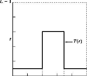
Fig.7. Slicing w/o background s=L-1; for A=< AB =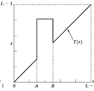

Fig.8. Slicing with background s=L-1; for A=< AB =

• IV.    Methodology

This paper implements a software program named PPI Analyzer to realize the above listed gray level image enhancement techniques. The developed software with its graphical user interface is created with MATLAB, short form for Matrix Laboratory. It is a fourth generation programming language which offers a multiparadigm environment for numerical computing. Apart from functions and data plotting and matrix manipulations MATLAB operation allows for implementation of algorithms, development of user interface, and providing interfacing for programs written in other languages including C, C++, Java, Fortran etc

MATLAB presents ideal environment suited to image processing [16]. Particular of such is the MATLAB's matrix-oriented language which is developed specifically for the manipulation of images, i.e. visual renderings of matrices. The outcome is an inexpensive and very easy way of manipulating operations of image processing. MATLAB possess in addition to image Processing Toolboxes, a powerful and interactive environment for processing and analysis of image and the performance varying calculations on images.

MATLAB presents several advantages in its operation to image processing. Key amount of them is the ability to obtain direct control to any portion of accessible information; what in most commercial image analysis systems would be highly impossible to perform. MATLAB makes it possible to halt any computation procedure at any specific point, make certain corrections or manipulations and then continue the computation at that point without affecting the overall programming code structure as it mostly occurs in other programming languages such C or C++ or undertaking the programming calculation from the beginning. Such ability is very useful for research and the development of new techniques and research analysis.

The software adopts a graphical user interface which among other qualities enables easier control of parameters and image operation techniques

PPI Analyzer is developed using MATLAB R2015a and run on Windows 8 operating system of x64 bit. Fig 10 illustrate a Screenshot of the vital Graphical user interface (GUI) of PPI Analyzer.

A flowchart to explain the operation of the implemented software is illustrated in Fig 9

To implement the techniques understudy, a novel pseudocode was written to implement and showcase the inner operations of each technique and how it performs and achieve its needed task.

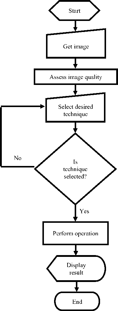
Fig 9. Flowchart of implemented software

Pseudo-code

• 1.    Get input image from user, p

• 2.    Assess the quality of image and convert to grayscale, p2 = (p(R)+ p(G) + p(B))/3

• 4.    Get selected operation command from user

• 5.    Initialize variables im = im2double(p2) set highest gray level, L = 256 compute c =(L - 1)/log(L)

• 6.    Perform operation

[m,n]=size(p2)

for i=1:m for j=1:n

Case 1: Image Negative compute the equation, s(i,j)=(L-1)-p2(i,j)

End

GOTO 7

Case 2:Power-Law Transform set arbitrary constant, c = 2 Get gamma, y value from user compute s(i, j) = c * im(i, j).^ y End

GOTO 7

Case 3: Log Transform compute s(i,j) = c*log(1+im) End

GOTO 7

• Case 4:    Inverse Log Transform

compute s(i,j) = exp(im^c)-1

End

GOTO 7

• Case 5:    Gray Level Slicing

compute using the condition if p2(i,j) >= 227

s(i,j) = 255;

else

s(i,j) = 0;

end if

End

GOTO 7

• Case 6:    Contrast stretching

• 7.    Display image

• 8.    Prompt user to save

• 9.    End

  

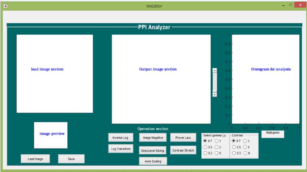
  Fig.10. Screenshot of PPI Analyzer User interface

  
  
  

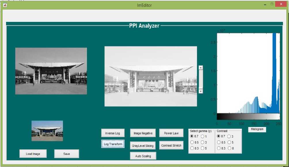
  Fig.11. Working environment of PPI Analyzer

  
  
  
  
  
  

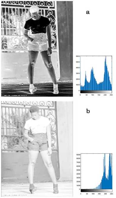
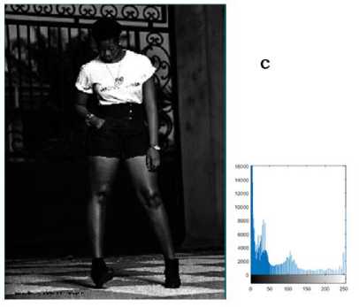
  Fig.12. Technique analysis of image (a – c)

  
  

set initial value for slope of the function, E and the mid-line to switch from dark values to light values, m m= 0.2

E=4

compute s= 1./(1+(m./(im2+eps)).^E)

Get update input of E or m from user update variables

End

GOTO 7

The PPI Analyzer has various section that perform needed task. The sections include the load image section, image preview, output image section, operation section and histogram interface. The load image section show selected grayscale image from the user, with the image preview showing the original image loaded by the user for operation and analysis. The output section displays the end result of a selected image after a technique has been selected. The portion of the histogram interface showcase the histogram of a selected image and its techniques to enable easy analysis of image technique and its variation. The operation section implements and details all gray-level techniques that is under consideration. The program also has a save button to enable storing of end result of image. Fig 11 illustrates the demonstration and working environment of the program implementation.

• V.    Simulation Experiment and Results

Various images with varying light intensity and contrast were passed through PPI analyzer to ascertain the correctness, operability and ability to achieve desired results. This section presents the experimental results

The main focus of the image negative technique is to achieve the reversal of image intensity levels in a manner which results in the production of the equivalent of a photographic negative. Log transform settles on mapping narrow range of image low gray-level values to wider range of output levels of which its opposite, inverse log dominates on expanding dark pixels values in an image while compressing the brighter-level values. From Figs 12 to 15, such objectives by each technique was attained through PPI Analyzer. From Fig 12, image a represent the result obtained for image negative, image b illustrates the image obtained after log transformation and image c display the end results after inverse transform. Each Fig also presents its histogram graph for further analysis.

The objective of Figs 13, 14 and 15 is to apply contrast stretching, power-law transformation and Gray level slicing respectively to the image.

Fig 13 and 14 illustrate the results obtained when a raw image was pass through the software to achieve contrast stretching of image and power law transformation

Image 1 of Fig 13 was obtained using slope function, E = 4 and a mid-line switch to control low to high pixels, m = 0.7. Image 2 was obtained after adjusting the controls of contrast, E = 8 and a mean value, m presented by selected image.

Fig 14 image 1 was the result of gamma correction value 0.7 and image 2, was with the gamma value 3. Both display varying gray-level intensities.

Fig 15 illustrates the result obtained from a raw image after passing through the PPI analyzer. The implemented technique was gray level slicing. From Fig 15, it can be noticed that the image background has been suppressed and the foreground image enhanced.

The level of darkness is very low such that, the histogram presents nothing in its frequency of gray level distribution.

On the whole, it can be noticed that from Figs 12 – 15 all the images have varying degree of color intensity or contrast, alluding to the application of each technique to achieve desired image.

PPI analyzer returned desired results effectively and efficiently without distortions or errors.

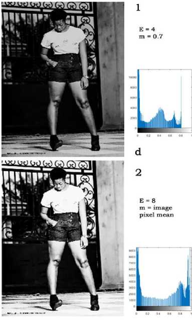
Fig.13. Contrast stretch implementation

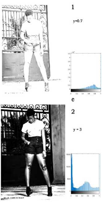
Fig.14. Power law transform implementation

• VI.    Conclusion

In this paper, an implementation of a computer and engineering based programming language, MATLAB, was used to implement six well known gray level techniques with a functional interactive graphical user interface. The study also presented the procedure needed to implement the various techniques understudy. The application presents a much more expedient way to achieve needed gray level output and a histogram interface for further analysis of loaded data. The implemented software solution demonstrate its ability to contain and return desired output of user. Despite the effectiveness and robustness of the implemented program, there is some margin of improvement. In future, the study can be extended to implement and study other advance image enhancement techniques.

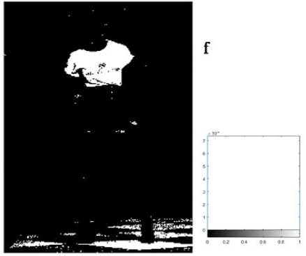
Fig.15. Gray level slicing implementation