Improved plant parenchyma extraction technology using artificial intelligence algorithms

DOI:

The previous paper "Extraction of plant parenchyma by computer image processing technology" mentioned the method of using image processing and other computer vision-related technologies for extraction of plant parenchyma [1]. This paper analyzes and verifies

the effectiveness of the algorithm through experiments. Discuss how to separate the morphology of axial parenchyma from a binary image containing only axial parenchyma and ducts. After analyzing the characteristics of axial parenchyma and catheter, an extraction algorithm based on the area histogram of the closed area was finally proposed. And it is verified by experiments that the effect of this method is better. Finally, this article is a summary of the axial parenchyma extraction algorithm, and at the same time analyzes the shortcomings of this algorithm, and also points out the future research direction [2].

With the rapid development of computer vision technology and wood science and technology, the application of computer vision technology in the field of wood science will surely develop further.

The study of axial parenchyma will become more and more extensive, and the corresponding characteristics of axial parenchyma will be established. The characteristic parameter table will better analyze the relationship between axial parenchyma and tree species [2-4].

With the deepening of research, the extraction technology of axial parenchyma is bound to become more and more developed, so as to achieve the purpose of intelligent identification, and a perfect software system will be established to replace manual identification of wood.

EXPERIMENTAL RESULTS AND ANALYSIS

Analysis of experimental results of image denoising processing

The median filter is filtered with a window containing an odd number of pixels, and the shape and size of the window will have a significant effect on the filtered result [4-7]. The effect of median filtering can be achieved by selecting a suitable window and processing it with equation. Generally, the size of the window is 3*3, 5*5, 7*7, 9*9, etc. What is the right size? In this paper, we use these window sizes to median filter the images, and the processed images and grayscale histograms are shown in figure 1 and figure 2, respectively.

From the histograms, we can analyze that there are several peaks and valleys in the histogram after the 3*3 and 5*5 templates, which is not conducive to the determination of the binarization threshold of the image. The peaks of the image histogram with the 9*9 template are sharper than the peaks of the image histogram with the 7*7 template. Therefore, it can be said that the median filtering of the image with 9*9 as the template is more effective.

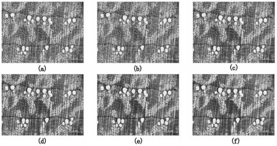
Figure 1. The demonstration diagram of median filtering in the Castanopsis megaphylla Image: (a) Original wood microscopic images; (b) Noise image after adding salt and pepper;

(c) Image after filtering processing as a template of a 3*3 model; (d) Image after filtering processing as a template of a 5*5 model; (e) Image after filtering processing as a template of a 7*7 model; (f) Image after filtering processing as a template of a 9*9 model.

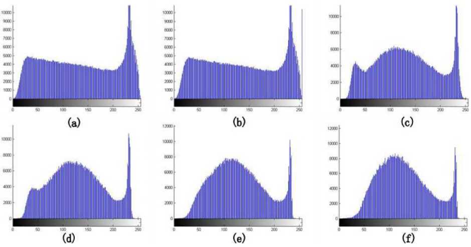
Figure 2. Gray histogram of median filtering in the Castanopsis megaphylla image: (a) Gray histogram of original wood microscopic images; (b) Noise image after adding salt and pepper; (c) Gray histogram after filtering processing as a template of a 3*3 model; (d) Gray histogram after filtering processing as a template of a 5*5 model; (e) Gray histogram after filtering processing as a template of a 7*7 model; (f) Gray histogram after filtering processing as a template of a 9*9 model.

Analysis of experimental results after the binarization process

Using equation (12) from [1], the threshold value of the grayscale image can be calculated, and then the image is transformed into a binary image, and figure 3 and figure 4

show the effect of the binarization process.

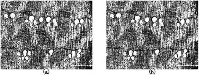
Figure 3. The effect chart of overall binary processing and block binary processing: (a) Image after overall binary processing; (b) Image after block binary processing.

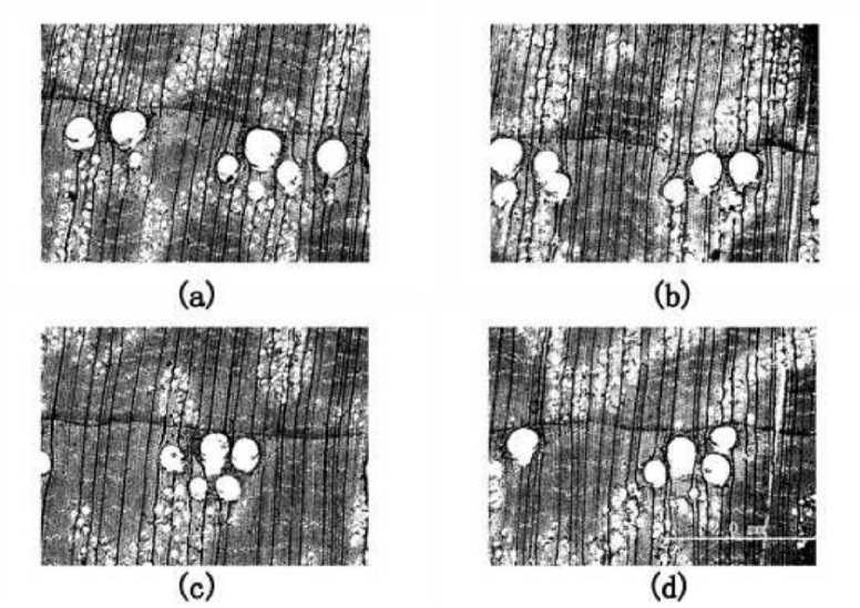
Figure 4. The effect chart of block binary processing: (a) Threshold is equal to 139; (b) Threshold is equal to 137; (c) Threshold is equal to 137; (d) Threshold is equal to 139.

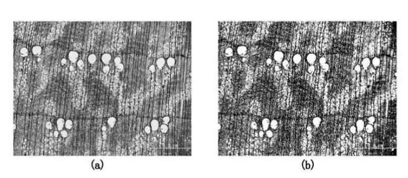
Figure 5. The comparison of effect:

• (a) wood microscopic image; (b) The image after binary processing.

Figure 4 (a) shows the effect of global thresholding with a threshold of 137, 139, 137, 137, 136 are the thresholds for each image after binarization, and each image must be merged into one after binarization to facilitate subsequent image processing. The merged image is shown in figure 4 (b). A closer look at (a) and (b) in figure 3 shows that the white area in figure 4 (b) is less than that in figure 4 (a). In this paper, we also calculate the area of the white area in figure (a) and figure (b) are 501148 and 500544 respectively (area is defined as the number of pixels), and it is obvious that the area of the white area in figure (b) is smaller than that of the white area in figure (a). Therefore, the binning binarization can be used to calculate the area of the white area in figure (b). Therefore, the chunked binarization can better filter out the other morphologies in the image, which is beneficial to retain the extraction of axial thin-walled tissue and duct morphology [8-13].

In figure 5, it can be seen that after the binarization process, the morphology of the axial thin-walled tissue and ducts is more evident, which facilitates the subsequent processing of the images using mathematical morphology and the successful separation of the morphology of the axial thin-walled tissue and ducts.

Analysis of experimental results after expansion and corrosion

After the noise reduction and image binarization, the features of axial thin-walled tissue and ducts in the wood micrographs are more prominent. From (b) in figure 3, it can be seen that there are some other tissue features, such as wood fibers and wood rays, in addition to the axial thin-walled tissue and ducts on the image [14-17]. Therefore, suitable structural elements can be selected to match the central block, and the objects in the image can be processed with expansion and erosion operations to achieve the extraction of axial thin-walled tissues and ducts.

After several experiments, it was found that the structural elements shown in figure 6 were selected to expand the image (b) in figure 5. The result is shown in figure 7.

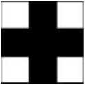
О I о

5?= I I I

О I 0

Figure 6. Structure element Se .

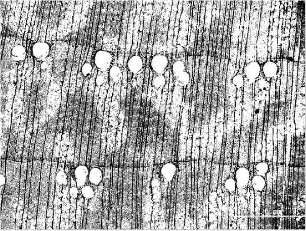
• Figure 7. Result of expansion operation.

As can be seen in figure 7, after the expansion process, the features of the axial thinwalled tissue and ducts are further enhanced, and the black-and-white effect of the image is more obvious. The axial thin-walled tissue and duct morphology are obviously thickened, and the following structural elements can be used to erode the image, "refine" or "shrink" the image after the expansion process, so as to separate the axial thin-walled tissue and duct morphology.

After several experiments, it was found that it was better to select a disc-type structural element with a radius of 8 for the corrosion operation of figure 7, and the treated result is shown in figure 8.

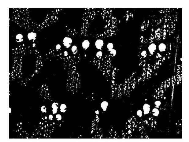
Figure 8. Result of erosion operation.

From figure 8, it can be found that there are many features on the wood cross-section, in addition to ducts and axial thin-walled tissue, there are also wood rays and wood fibers, etc. The corrosion operation filters out the other features, leaving only the features containing only axial thin-walled tissue and duct morphology. In the process of corrosion operation [18-22], the effect of different radii of the disc-type structural elements is different, the effect is shown in figure 9.

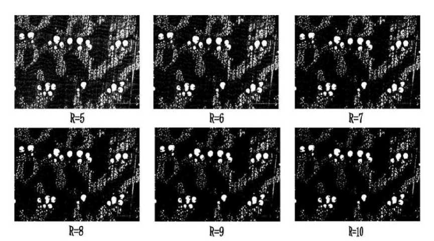
Figure 9. The effect of processing image of using different radius’ structural element.

In this paper, the experiment was carried out by increasing R=1 in order, and it can be found from the above figure that the effect is better at R=8. From figure 8, we find that the morphology of axial thin-walled tissue and ducts have basically been extracted, and the results are still better. In the above series of discussions, we have focused on the microscopic images of large leaf cones [23-26], and then the distribution of axial thin-walled tissues and ducts varies greatly among different tree species, so whether the algorithm in this paper can be applied to different tree species will be discussed in the next section.

Experimental results and analysis of the extraction effects of different tree species

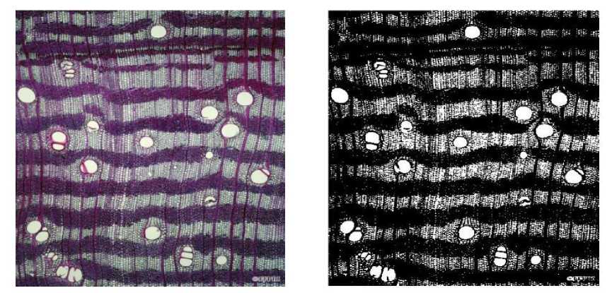
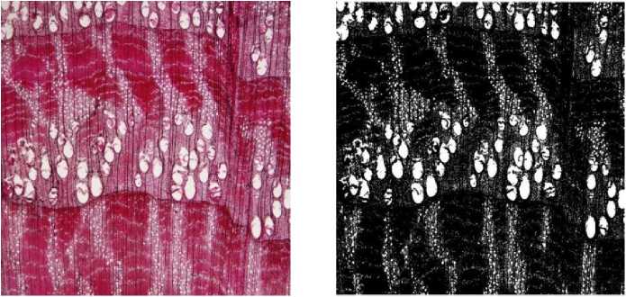
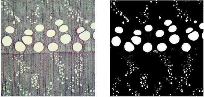
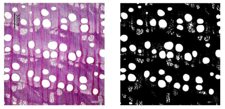
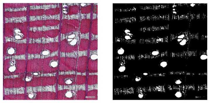
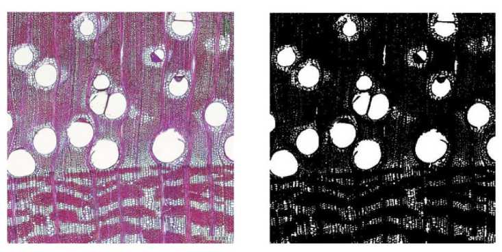
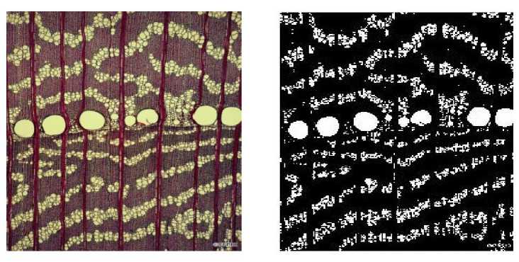
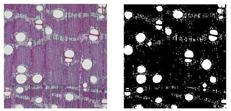
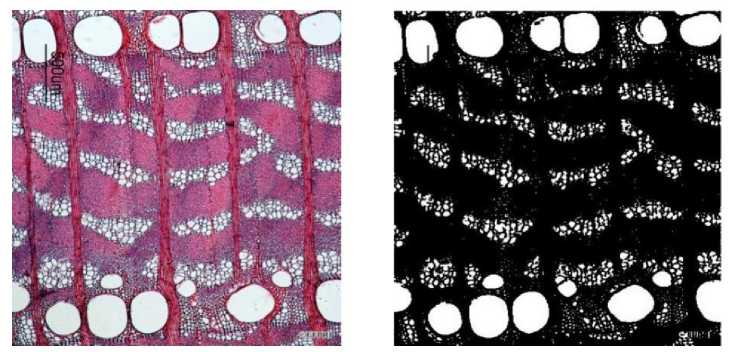
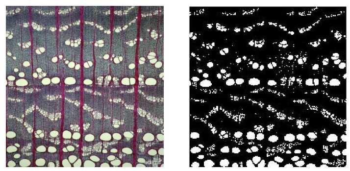
The algorithm shown in pervious paper was used to process the microscopic images of 10 wood cross-sections, and good results were obtained for all of them. good results. Figure 10 shows the cross-sectional microstructure images of the 10 wood species, as well as the comparison of the axial thin-walled tissue and conduction.

The comparison of the cross-sectional microstructure images and axial thin-walled tissue and conductor morphology of the 10 species is shown in figure 10. These 10 species are: water bark, chinkapin, Japanese millet, broussonetia, tianxian fruit, sapodilla, rowan, brown leaf tree, beech, and narrow leaf park.

(a) Hydrocotyledon.

(b) Rice chink.

(c) Japanese corn.

(d) Broussonetia.

(e) Tian Xian Guo.

(f) Sapindus.

(g) Catalpa.

(h) Rough-leaved trees.

(i) Beech tree.

(j) Narrow-leaved Park.

Figure 10. Microstructure images and results of axial parenchyma and pores Segmentation.

Table 1. The comparison of using different shapes and sizes structural element for different tree species.

Structural elements during expansion Т   CHPPWK				Structural elements during corrosion
	Shape		Size	Shape	Radius
Water yellow skin	Figure	10	3*3	Disc-shaped	R=2
Quercus chinensis	Figure	10	3*3	Disc-shaped	R=4
Japanese corn	Figure	10	3*3	Disc-shaped	R=5
Broussonetia	Figure	10	3*3	Disc-shaped	R=4
Tian Xian Fruit	Figure	10	3*3	Disc-shaped	R=4
Sapindus	Figure	10	3*3	Disc-shaped	R=3
Catalpa	Figure	10	3*3	Disc-shaped	R=3
Rough Leaf Tree	Figure	10	3*3	Disc-shaped	R=4
Beech Tree	Figure	10	3*3	Disc-shaped	R=3
Narrow-leaved Park	Figure	10	3*3	Disc-shaped	R=3

The comparison of the left and right images in figure 10 shows that the morphology of axial thin-walled tissue and ducts has been successfully separated from the original image of wood by the present algorithm processing. It can also be found in the figure that some wood microscopic images may be acquired with incomplete morphology of the axial thin-walled tissue due to external factors, as in figure 10(i). Therefore, the quality of wood microscopic images also affects the extraction effect, and good quality images will make the extraction better, which also facilitates the analysis and understanding of the images. From table 1, we can see that the shapes of the selected structural elements are the same for the morphological processing of these different species [23-27], but the sizes of the selected disc-shaped structural elements are different for the erosion operation. In short, processing different wood images, as long as the selection of the appropriate radius of the circular structural elements, you can get good results. After several experiments, we found that the radius of the disc-shaped structural element is between 1 and 10 when the image is corroded with the disc-shaped structural element for the extraction of axial thin-walled tissues and ducts. The results are better when processed between here and there. The morphology of the axial thin-walled tissue and the ducts have been extracted, and the next step is to successfully extract the axial thin-walled tissue by filtering out the ducts from them. How to filter out the ducts will be discussed in the next chapter.

Summary of this chapter

This chapter focuses on the extraction methods of axial thin-walled tissues and ducts in wood cross-section micrographs. Firstly, it introduces the methods of digital image segmentation and analyzes the advantages and disadvantages of commonly used digital image methods, secondly, it proposes a morphology-based extraction method by combining the distribution characteristics of axial thin-walled tissues and ducts in wood cross-section microscopic images and previous research on wood identification, and finally, through experimental analysis and verification, the algorithm is able to effectively extract the morphology of axial thin-walled tissues and ducts in wood microscopic images.

EXTRACTION OF AXIAL THIN-WALLED TISSUE BASED ON AREA HISTOGRAM OF CLOSED AREA

In this Chapter of the paper, the extraction method of axial thin-walled tissue and ducts of wood based on mathematical morphology has been proposed, and it has been experimentally verified that the method can successfully extract the morphology of axial thin-walled tissue and ducts from the wood cross-section microscopic images.

The wood image has been processed by the algorithm in the previous chapter, and although some other wood grain features have been filtered out, the morphology of the ducts has not been filtered out. Next, as long as the morphology of the ducts is filtered out from the binary image, then the axial thin-walled tissue can be separated independently. Therefore, in this paper, we propose an axial thin-walled tissue extraction algorithm based on the area histogram of the enclosed area in combination with the knowledge of wood science. Since the area of ducts is much larger than that of axial thin-walled tissues, they can be easily distinguished by the area feature [28-31].

In this paper, we firstly label the closed areas in the binary images containing only conduit and axial thin-walled tissue morphology, secondly calculate the area of these already labeled closed areas, and then draw a histogram of the area of closed areas to determine the area threshold from which the axial thin-walled tissue is successfully separated. The whole processing flow of the algorithm is shown in figure 11.

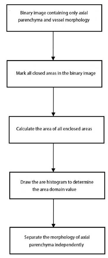
Figure 11. Flow char for the extraction of axial Parenchyma.

Label all closed regions in the binary image

To obtain the area of closed regions in binary images containing only axial thin-walled tissue and duct morphology, it is necessary to label these closed regions to facilitate the calculation. There are two general ways to label closed regions in binary images: four-neighborhood and eight-neighborhood. Suppose a pixel p in a binary image has the coordinates (x,y), and each pixel has two horizontal and two vertical pixel points, then the coordinates of the two horizontal and two vertical pixel points of pixel p with coordinates (x,y) are (x,y+1), (x,y-1), (x+1, y), and (x-1,y), respectively. n1(p) is defined as the set of these four neighboring pixels of p, as shown in the black shaded part in figure 12(a). N2(p) is defined as the set of these four neighboring pixels of p in the diagonal direction, as shown in the black shaded part in figure 12(b). The concatenation of N1(p) and N2(p) is the set of eight neighbors of p, denoted as N3 (p). The set of N1(p) and N2(p) is the set of eight neighbors of p, denoted as N3 (p), as shown in the shaded part in figure 12 (c).

In this paper, we use 8-neighborhoods to label all closed regions in the binary image, and the pixels in each different closed region are assigned to a unique integer ranging from 1 to the total number of pixels in each different closed region are assigned to a unique integer ranging from 1 to the total number of closed regions [32-36]. That is that is, the pixel with marker value 1 belongs to the first closed region; the pixel with marker value 2 belongs to the second closed region; and so on to obtain the corresponding marker matrix and the total number

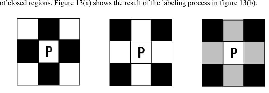
Figure 12. Four neighborhood and eight neighborhoods:

(a) Pixels P and four neighborhoods; (b) Pixels P and four diagonal neighborhoods;(c) Pixels

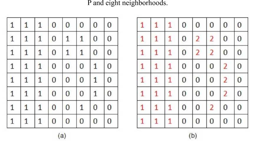
Figure 13. The demonstration diagram of making the closed area

(a) Binary image; (b)The effect is obtained by using the 8 neighborhoods.

Calculation of the area of the closed area

After the algorithm from the previous chapter of this paper, the wood microscopy image contains only the axial thin-walled tissue and duct morphology, and the image is a binary image at this point. After labeling all the closed areas in the binary image as in the previous section, we can count the area of each closed area by using the pixel-counting area method. As the name suggests, this is a relatively simple method of calculating the area by counting the number of pixels in each enclosed area.

After extracting the axial thin-walled tissue and ducts, a binary map containing only these two morphologies can be obtained [34-37], and the axial thin-walled tissue and duct morphological regions in the binary image are labeled as 1, while the other parts are labeled as 0. Assume that after labeling, the number of closed regions is n, and the number of 1, 2, 3 ......n in the labeling matrix is a1, a2 and a3......an (whose initial values are all 0). By scanning the values of the matrix one by one, a1 is added 1 for each value of 1, a2 is added 1 for value of 2, a3 is added 1 for value of 3, a4 is added 1 for value of 4, and so on. The values of a1, a2, a3, a4, a5 ......an are the area of each enclosed region. The area S of the enclosed area can be calculated from the following formula.

5 = £1

U-yep)

In Equation (1), p is the point with a pixel value of 1. The area S is the total number of pixels in the enclosed region. This method is not only simple, but also has a small error, and is the best estimate of the area of the original closed region.

Area histogram

A histogram is a graph that represents the distribution of data using a series of rectangles of equal width and unequal height. The width of the rectangles indicates the interval of the data range, and the height of the rectangles indicates the frequency of the data within a given interval. The function of the histogram is to facilitate the analysis of the distribution pattern of a quality characteristic; to convey information about the fluctuation of the process state; and to facilitate people to determine where to make quality improvements [35-38].

In the binary image containing only axial thin-walled tissue and ducts, by analyzing the respective distribution characteristics and morphological features of axial thin-walled tissue and ducts, it was found that the area of axial thin-walled tissue to ducts varied greatly, so by calculating the area and drawing a histogram, and then by using the histogram, the area threshold could be visually determined, and then they could be distinguished.

In this paper, instead of simply displaying the area of all the closed areas calculated above directly in a histogram, all the areas are reduced to between 0 and 255, and the maximum value of the area of these closed areas must be reduced to 255, and all are expressed as integers (rounded off). If the maximum value of area is a, then all the area thresholds are divided by T (T=a/255), so that all the areas can be reduced to between 0 and 255. In this paper, we use the matlab software to analyze and process the images. After the above processing, we can directly use the function imhist in Matlab to display the histogram, which saves the time of data processing; secondly, the area of the closed area less than 255 will be reduced to 0, which can increase the difference between the closed area of axial thin-walled tissue and the closed area of the duct in the histogram. In conclusion, the axial thin-walled tissue can be better separated from the catheter.

Determination of the area threshold of the closed area

In the binary image containing only the duct and axial thin-walled tissue morphology, the area threshold can be intuitively obtained from the histogram because the area of the duct is much larger than that of the axial thin-walled tissue. From the theoretical analysis, it is known that the area of the closed area of the catheter will be biased to the right side of the coordinate axis, and the area of the closed area of the axial thin-walled tissue will be biased to the left side of the coordinate axis. After extensive experiments, it is also found that the number of catheters in an image can be roughly estimated as b. Then, the area of b closed areas can be found from right to left in the histogram, which is the area of catheters displayed on the histogram.

Separate out the axial thin-walled tissue

Once the area threshold of the closed area is obtained from the histogram, the closed areas larger than the threshold can be removed. Therefore, the original binary image is transformed into a labeled matrix after processing in the previous section, and then transformed into a binary image after processing by the method shown in this section, and the morphology of the ducts is also filtered out from the image. After a series of processing, the morphology of the axial thin-walled tissue was successfully extracted from the wood micrographs [38-40].

Assuming that the obtained area threshold is 10, then all closed areas with area greater than 10 are to be removed. After processing in figure 14(a), figure 14(b) is obtained.

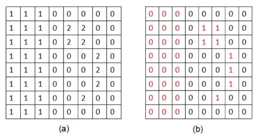
Figure 14. The demonstration diagram of removing large closed area: (a) Label matrix; (b) Binary image after processing.

Experimental results and analysis

Histogram of the area of the large leaf cone

For figure 8, the area histogram obtained by applying the algorithm described in this chapter is shown in figure 15.

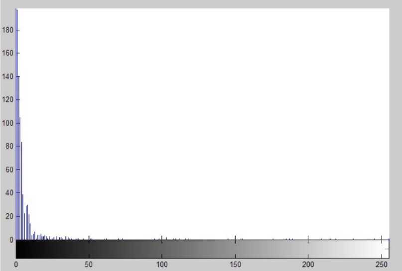
Figure 15. The area histogram of Castanopsis megaphylla closed area.

According to the area histogram, the area threshold is determined as ST=35*T=5190.2=5190 (if p is not an integer, it can be rounded up to an integer). Since the area of the closed area is divided by T when the histogram is drawn, the area threshold is multiplied by T to be the original area threshold of the closed area.

Analysis of experimental results after processing of large leaf cone images

With the area threshold determined above and the processing of the algorithm in this chapter, the result is shown in figure 16 below.

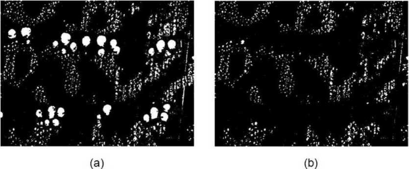
Figure 16. Original binary images and their results of axial parenchyma and pores Segmentation: (a) the images of axial parenchyma and pores; (b) the images of axial parenchyma.

As can be seen from the above figure, for the image of the large leaf cone, applying the algorithm in this chapter is indeed able to filter out the ducts from the axial thin-walled tissue, so that only the axial thin-walled tissue pattern is present in the image [41]. Whether this algorithm can also achieve good results for other wood images will be analyzed in the next subsection.

Analysis of experimental results of axial thin-walled tissue extraction from different tree species

Histogram of area thresholds and area thresholds for different tree species. For the binary images containing only axial thin-walled tissue and duct morphology for the 10 different tree species on the right side of figure 10, the area histograms of the enclosed areas obtained after processing by this algorithm are as follows.

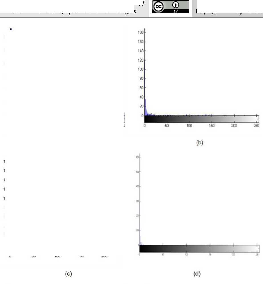
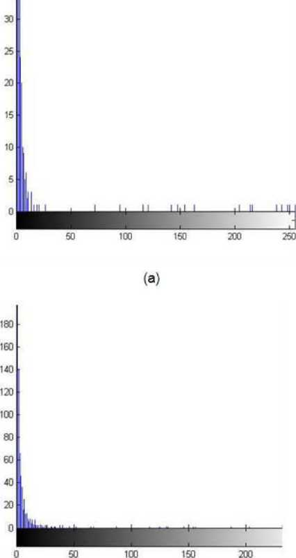
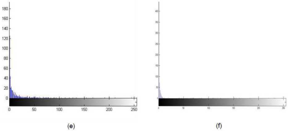
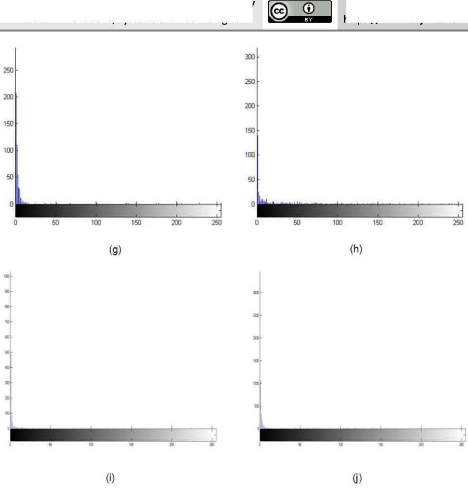
Figure 17. The area histogram of the closed area in the binary images of different species of trees: (a) Pongamia pinnata; (b) Castanopsis carlesii; (c) Castanea crenata Sieb; (d) Broussonetia papyrifera; (e) Ficus beecheyana Hook; (f) Sapindus mukorossi Gaertn; (g) Kalopanax septemlobus; (h) Aphananthe aspera; (i) zelkova tree; (j) jessoensis Koidz.

The closed threshold area thresholds determined from the area histograms above, are shown in table 2.

Table 2. The closed area threshold in the binary images of different species of trees.

Tree species name      Closed area thr eshold

Water yellow skin        2000

Quercus chinensis        2000

Japanese corn          1000

Broussonetia	700
Tian Xian Fruit	550
Sapindus	1500
Catalpa	6000
Rough Leaf Tree	2000
Beech Tree	2500
Narrow-leaved Park	1200

Analysis of experimental results for different tree species using this algorithm to extract axial thin-walled tissues. Based on the thresholds in table 2 and the algorithm described in this chapter, the effect of processing the image on the right in figure 10 is shown in figure 18.

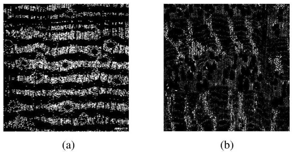
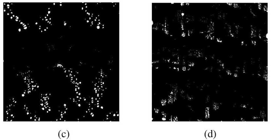
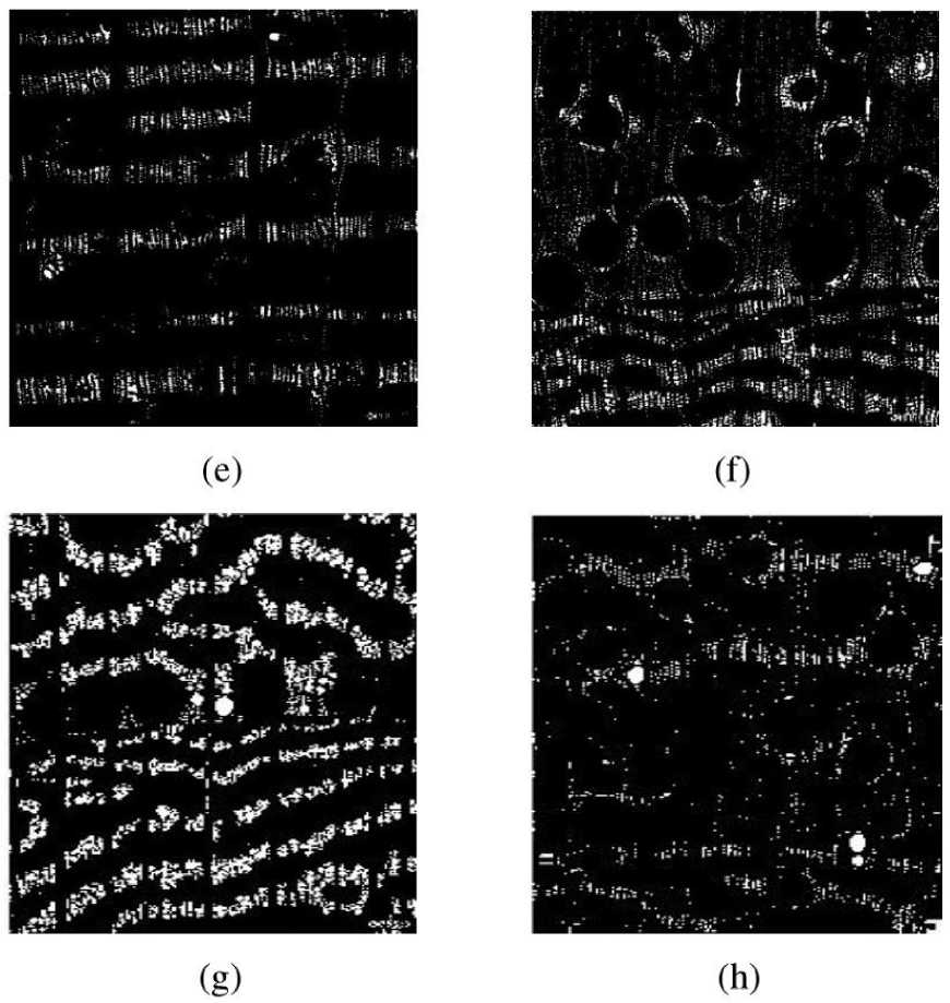
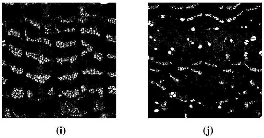
Figure 18. The results of axial parenchyma segmentation: (a) Pongamia pinnata; (b) Castanopsis carlesii; (c) Castanea crenata Sieb;(d) Broussonetia papyrifera; (e) Ficus beecheyana Hook; (f) Sapindus mukorossi Gaertn; (g) Kalopanax septemlobus; (h) Aphananthe aspera; (i) zelkova tree; (j) jessoensis Koidz.

After the original wood micrographs were grayed out, noise reduction, binarization, morphological processing, labeling the area of the closed area, calculating the area of the closed area, drawing a histogram to determine the area threshold, and filtering out the ducts, the final result is shown in figure 18.

Comparing figure 18 with the image on the right side of figure 10, it can be seen that the ducts have been filtered out and only the axial thin-walled tissue morphology remains. It can be said that the axial thin-walled tissue patterns can be successfully extracted from the wood micrographs for different species using this algorithm, which indicates that the method described in this paper is effective. However, there are various types of axial thin-walled tissues in broad-leaved wood [42], such as off-tube and on-tube in relation to the position of the ducts, and the aggregation of thin-walled tissues can be divided into scattered, whorled, winged, aggregated winged, banded, etc.

The method in this paper may have slightly different effects on the extraction of these different combinations of thin-walled tissues, but as long as the image is eroded and the area threshold is determined However, as long as the appropriate circular structure elements and accurate area thresholds are selected, this difference can be reduced and a good extraction effect can be achieved.

Summary of this chapter

This chapter focuses on how to extract axial thin-walled tissue from binary images containing only axial thin-walled tissue and duct morphology. Combining the knowledge of wood science and computer vision, this chapter explores the axial thin-walled tissue extraction algorithm based on the area histogram of the closed region, carefully analyzes each step of the algorithm and demonstrates it with effect pictures, and finally verifies that the algorithm is effective through experimental data analysis.

SUMMARY AND OUTLOOK

Conclusion of this paper

Combining the knowledge of wood science and technology and computer vision technology, this paper focuses on the morphological characteristics of axial thin-walled tissues in microscopic cross-sectional images of wood, and explores the algorithm for extracting axial thin-walled tissues of wood. In this paper, firstly, the image is pre-processed; secondly, suitable structural elements are selected, and the expansion and erosion operations of mathematical morphology are applied to extract the binary image containing only axial thin-walled tissue and duct morphology; finally, the axial thin-walled tissue is successfully extracted by analyzing the difference of features between duct and axial thin-walled tissue in the binary image and applying the idea of closed area histogram. When using the algorithm proposed in this paper to process some microscopic images, and through several experiments and analyses, we can obtain the following conclusions.

• •    When noise reduction is applied to the image by median filtering, generally 3*3, 5*5, 7*7 and 9*9 windows are used for filtering, but 9*9 is the best when the purpose is to extract thin-walled tissue in the axial direction.

• •    The distribution of axial thin-walled tissues is different in microscopic images of different tree species, and the distribution of axial thin-walled tissues is also different in different areas of microscopic images of the same tree species. Therefore, the global threshold value cannot meet the need in image binarization, and the effect of binarization in blocks is better for the extraction of axial thin-walled tissues.

• •    When the image is expanded, the 3*3 cross-shaped structural elements selected in this paper are more effective.

• •    In the image etching operation, a disc-shaped structural element is selected. Through a large number of experimental results, it is found that the radius of structural elements is generally distributed between 1 and 10, so that the extraction effect is the best. The 11 species selected in this paper are: water yellow bark, chinaberry, Japanese millet, kozo, tenebrion, sapodilla, rowan, brown leaf tree, beech, narrow leaf park and big leaf cone. The radii of selected disc-shaped structures were: 2, 4, 5, 4, 4, 3, 3, 4, 3, 3, 2, and 8, respectively.

• •    The method of closed area histogram can visualize the area difference of axial thinwalled tissues and ducts, so as to determine their area thresholds and achieve a good segmentation effect.

Next research directions

The core of this paper is to investigate the characteristics and extraction techniques of axial thin-walled tissue in microscopic cross-sectional images of wood, although this paper has explored an axial thin-walled tissue extraction algorithm, done a lot of theoretical research, and verified the effectiveness of the algorithm through experiments. However, there are still shortcomings [43-45], and there are many excellent and more intelligent algorithms worthy of our study and research, therefore, the following points are the direction of our future research work:

• •    Improve the quality of the original wood microscopic images. In the study of axial thin-wall extraction techniques, we can know that the quality of wood microscopic images, can affect the effect of axial thin-wall extraction, which is detrimental to the analysis and understanding of the images. Wood microscopic images are obtained by making slices and observing them with a microscope, which generates a lot of noise in the process, how to reduce this noise and obtain higher quality wood microscopic images? The above mentioned will be further researched in the future.

• •    Collect microscopic images of wood from different tree species. If we have microscopic images of wood from many species with good quality, it will be easier to study the extraction of thin-walled tissue in the axial direction.

• •    To explore intelligent methods of selecting the size of structural elements. This paper does not introduce an intelligent method for selecting the size of disc-shaped structural elements. How to determine the size of this radius intelligently for each image, which can save a lot of time and improve the efficiency, is also a problem we

need to study in the future.

• •    Efficient and intelligent axial thin-walled tissue extraction algorithm. The effect of using this method for different images will definitely be different. Therefore, how to extract the axial thin-walled tissue quickly and effectively for the unused images is a major direction for future research [46-48].

In summary, this paper explores the extraction algorithm of axial thin-wall by combining the texture features of some microstructure images of wood. This paper introduces computer vision technology to the study of axial thin-wall tissue of wood, which is rare at present, and provides a possibility for better study of intelligent axial thin-wall tissue extraction technology in the future, and also provides a new way for intelligent recognition of wood.