Improved PSO tuned Classical Controllers (PID and SMC) for Robotic Manipulator

Published Online January 2015 in MECS DOI: 10.5815/ijmecs.2015.01.07

Despite the success of modern control theory, Proportional Integral Derivative (PID) and Sliding Mode Controller (SMC) are the two earliest control techniques that are still used widely in almost all the industrial applications. This is because of their simplicity, easy to implement in hardware or software, and does not require a precise process model to start up and maintain and hence has invariance to parametric uncertainties [1-3]. Most crucial step for achieving a good performance t in PID and SMC is finding out the optimal values of the constant parameters. In PID controller, constants of the controllers have to have a higher value for good control action [4]; but also increasing their value can take the controller to the instability. In SMC, constant of switching function and exponential reaching law are important. In SMC, t = —Лs — Sg g n(s) (Л > 0, к > 0) , [5] value of k should be small to eliminate chattering and should be kept large to increase the robustness of SMC. Increasing A can increase the reaching velocity but can cause chattering in SMC. With this discussion it can be said that for a good control performance the basic necessity is to get an optimal value of these parameters of PID and SMC.

Tuning methods of classical controllers can be classified as traditional and intelligent methods. Traditional methods include Trial And Error (TAE) methods by which it is very hard to find the optimized tuned parameters. Also in contrast to intelligent methods, TAE tuning method is very time consuming and a frustrating job [jref].

Other than tuning problem, some other problems in SMC are discussed further. Firstly, the key technical problem of chattering in SMC is a challenging issue. Undesirable phenomenon of oscillations with finite frequency and amplitude around a predefined switching manifold is known as ‘chattering’ [7]. This condition of chattering may worsen further if some unmodeled dynamics of the system comes into picture. Chattering can increase the controller burden and damage the controller parts. Secondly, the stage from initial state (i.e. reaching stage or non-sliding stage) to sliding state system is only a feedback controller and hence robustness of the system is weakened to a great extend [8].

In literature, many solutions like boundary layer solutions [9], continuous approximation method [10] and second and higher order SMC [11] have been proposed for chattering reduction. One of the boundary layer methods is to replace pure signum function of SMC with Pseudo Sliding Function [12].

Robotic manipulator is highly reliable and most commonly used advanced factory equipment these days. An n-link robotic manipulator is a complicated system with highly non-linear dynamics, strong coupling and the uncertainties in the dynamics like payload mass, disturbance and friction etc. Hence, it can be said that it is almost impossible to get an accurate mathematical model of a manipulator. Hence, the challenge is still to design an effective controller with accuracy and without the accurate knowledge of the system dynamics. One solution to the problem is to make the classical controllers intelligent. This can be achieved by introduction of intelligent agents to the classical controllers like PID and SMC. An intelligent technique like Particle Swarm Optimization (PSO) is capable to make smart optimizations in nature [13]. Hence, diffusion of intelligent techniques like PSO with PID [14-17] and SMC [18-22] has become a major research topic recently and achieved a lot of success in last few years.

The rest of the paper is organized as follows-Section II describes the dynamics and the properties of the robotic anipulator system, Section III explains the concepts of the particle swarm optimization Section IV has the elementary concepts of the proportional integral derivative controller followed by sliding mode controller basics in the Section V which is followed by simulation examples. Finally Section VI gives the conclusion.

• II.    System Model And Dynamics

• A.    Dynamics of the Robotic Manipulator

The dynamics of revolute joint type n-link robot can be described by following nonlinear differential equation [23], given in (1)

M(q)q̈+V(q, q̇) +G(q) +dist=Т     (1)

with q є Rn as the join position variables,

τ є Rn as vector of input torques,

M (q) є Rnxn is the inertia matrix which is symmetric and positive definite,

V(q, q̇) є R^nxn is the coriolis and centripetal matrix,

G (q) є Rn includes the gravitational forces and dist є Rn is the any disturbance (like payload changes, friction or noise etc.) in manipulator.

• B.    Properties of the Robot Manipulator

Property 1. The inertia matrix M(q) is symmetric and positive definite and satisfies m17n ≤М(q)≤m2/n ,∀ qє Rn        (2)

where тг and m2are positive constant, and  єR nXn is the identity matrix.

Property 2. The coriolis and centrifugal matrix V(q, q̇) satisfies

‖V(q, q̇)‖ ≤ Tc ‖ q ‖ , ∀ q , ̇є Rⁿ ,           (3)

where T_c is a positive constant and ‖(․)‖ is the Euclidean norm.

Property 3. The gravity term is bounded as

‖G(q)‖ ≤ g_b , ∀ q є Rⁿ ,              (4)

where 9ъ is a known positive function of q.

Property 4. Using a proper definition of the matrix V(q, q̇) the к̇(q)-2V(q,q̇) is a skew symmetric and satisfies xT [ḃ(q) -2V(q, q̇)]x=0, ∀Xє Rn .        (5)

• III.    Particle Swarm Optimization

• A.    Basic PSO

  Particle Swarm Optimization (PSO) algorithm is developed by Kennedy and Elbe hart in 1995 [24]. PSO is initialized by population of random solutions called as particles and updating themselves continuously. A velocity vector is used to update the current position of each particle in the swarm. Each particle keeps a record of its coordinates and fitness value related to the best solution achieved so far in the population space. This value is named as personal best. Another best value named as local best is the best value obtained so far by any particle in the neighbor of the particle. Considering all the particles as the topological neighbors, the best position is called as the global best. At each step velocity of the particle changes as in (5 & 6) and moves towards its personal best and local best. Every component of the velocity is weighted by a random term which assures the exploration of problem space. This process is iterated a set number of times or until a specified criterion is met.

Vid =     ⁺C ^∈ 1⁽ Pid ^- Xu )+ C ^∈ 2( Pxd ^- Xu )   (5)

Xu =    ⁺ Vu              (6)

where, in a d-dimensional space ⃗⃗ =(■^11 , ■^12 ,… X[d ) is a present position vector, ⃗⃗ =( Pil , Pi2 ,… Pid ) is a best position vector, ⃗ ⃗ ⃗ =(^il , ^12 ,… ^id ) is a velocity vector, c is a constant having value 2, ∈ and ∈ 2 are the random number generators.

• B.    Modified PSO

Particle Swarm Optimizer has better computational efficiency, requires less memory, less number of parameters to adjust. PSO works for both analog and digital systems. Also, although the basic PSO has been found a good optimizer but still a lot research and work has been done in literature to improve the performance of the basic PSO.

A fixed value of v max is not applicable to all the search problems. As a larger value of v_max facilitates global search while smaller value of v_max facilitates the local search. For this, Shi and Eberhart in 1998 [25] proposed an inertia weight ‘w’ to have a better balance between the local and global search. Use of this ‘w’ has improved performance in many applications. With this weight inertia ’w’, (5) can be written as (7)

Vu =      ⁺C ^∈ 1⁽ Pid ^- Xu )+ C ^∈ 2( Pxd ^- Xu ) (7)

With a proper selection of ‘w’ number of iterations also reduces. For a particle swarm optimization problem a better global search in starting phase help the algorithm converge to an area quickly and then a stronger local search is required to get a high precise value [26]. Hence, it is required to keep the value of ‘w’ varying and linearly decreasing. Value of w which can be used as in (8)

W=( ^max ^- ^min ₎ (        ) ₊ ^min     (8)

\ tLermax / where wmax and wmin are maximum and minimum values of the inertia weight, iter is the current iteration and itermax is the maximum number of iterations.

In PSO, updated speed of a particle after every iteration must be less than a specified value (v max ). This is to prevent particle to be driven to a high speed; which can take the particle towards the boundary of the design and after this the search pace cannot be searched properly. Limits for the initial velocity are taken between upper and lower bound of the variables to be optimized. If this velocity limit remains unchanged, a large value of velocity in later iterations may slow down the convergence process. Hence, as proposed by [27] a gradual reduction of velocity is required. So, velocity ranges U max and ^ min taken in this paper is given in (9 & 10) below

^ max =0․1∗( ^ max - ^min ) (9)

^ min =-0․1∗( ^ max - ^min ) (10)

where ^ max and ^ min are the upper and lower limits of the parameters to optimize. Initial value of the parameters are taken as in (11 & 12)

^ init ^ min +( ^ max

~ ^ min )∗e

PID controller is a generic control loop feedback mechanism widely used in industrial control systems. PID is the most commonly used feedback controller. The controller attempts to minimize the error by adjusting the process control inputs. General equation for PID controller is given in (17).

т =    (t)+К_й ̇(t)+Ki ∫e(t)        (17)

where, Kp , Кд and K[ are suitable positive definite diagonal n x n matrices.

Simulation Example 4.1:

To check the effectiveness of the classical PID controller, it is applied on a two link robotic manipulator whose parameter matrices for Eq. (1) are as follows [28].

M(q) =*m11 m +

21    22

V(q,q̇)q̇=*:21 ⁺

G(q)=[^s₈21 ^]

where

^pinit ^ min +( ^ max

~ ^min )∗ ^e

The controller design problem can be defined here as; given the desired trajectory q d with some system parameters being unknown, the aim is to derive a control law for the torque input т ; such that the position vector q can track the desired trajectories and error vector e tends to 0.

Let the tracking error vector be defined in (13) as e=q-qd ,є ^”

And then the velocity error vector is given as in (14)

e ? = qa -q>eRn(14)

Qi =0․3sin(0․7t-) +0․3sin(0․1t-)+0․7(15)

Я2 =0․5sin(0․9t-)+0․5sin(0․1t-)+1․1(16)

The sampling time is taken as 0.01 for the whole simulation.

m11=(m₁ + m₂ ) af + m!^ +2 771-2 ^-T'1^7'2 cos q₂

m12=m₂a^ + 777-2 ^1 ^2 cos q₂ =  21

77722=m2a| v11=-m1a1a2(2q̇1 q̇ 2 +q̇2)sinq2

21=maaq̇sinq g11=(m1+m2)ga1cosq1 +m2 ga 2 cos(q1 +q2)

921=m2 ga 2 cos(q 1 +q 2 )

where m and m 2 are the mass and a and a 2 are the lengths of the links 1 & 2 respectively and g is the gravity acceleration.

In order to testify the performances of the TAE and proposed PSO tuned PID controller; parameters of the manipulator model have been taken as:

m 1 = 1kg ; m 2 = 1kg ; a 1 =a 2 =1m ; g = 9․8m/s²

Values of the controller gains for PD controller by TAE are taken as

500   0         50  0        25  0

K =* _{0   120} + ; K^d =* _{0   13} + ; K‘ =* _{0   25} + ;

• IV.    Proportional Intergral Derivative (pid)

For a payload mass change (m 2 +∆m) of 35% rise in the mass of joint 2 of the manipulator results for the proposed and the classical PID control schemes have been represented in Figs. 3 & 4. Fig 5 & 6 represents the tracking errors for joint 1 & 2 for the controllers without and with payload changes.

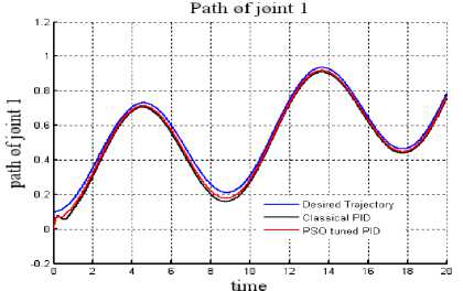
Fig. 1: Trajectory tracked:Joint 1(without payload).

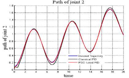
Fig. 2: Trajectory tracked:Joint 2(without payload).

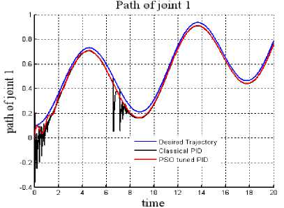
Fig. 3: Trajectory tracked:Joint 1(with payload).

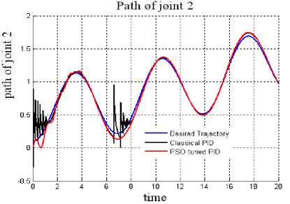
Fig. 4: Trajectory tracked:Joint 2(with payload).

Table 1. MSE of Tracking Error for Classical and Proposed PID

Controller	without payload		with payload
	Joint 1	Joint 2	Joint 1	Joint 2
Classical PID	0.0015	0.0018	0.0034	0.006
PSO tuned PID	7.87E-04	0.0047	0.0081	1.98E-04

• V.    Sliding Mode Controller (smc)

The conventional sliding mode control used sliding function definition involving the position error and the velocity error of the form (18)

s( t )= ̇+Ʌ!e               (18)

In this paper, the sliding function is extended to include the integral error term and the SMC which is including PID part is designed and its stability guarantee has been proven in [29, 30]. Sliding function with integral action is defined in Eq. (19)

s( t )=(̇+Ʌ ! e+Ʌ₂∫ e dt         (19)

where Ʌ2_ and Ʌ2 are constant positive definite diagonal matrices [31]. Hence, s=0 is a stable sliding surface and e →0 as t → ∞ .

Torque Eq. (20) for SMC as defined by Kuo [30] is

• T=- M ( ∧ ! ̇+ ∧ 2 ⁶- ̈ ;d )+ V ( ̇ Cl - ∧ i e-

• Λ2∫ e dt)+G- Xs -К-Td           (20)

where A= [a1, a2…..an], a is a positive constant, and Eq. (21) is given as

К =- к sin( s )               (21)

where k: a positive constant that represent the discontinuous constant gain;

T d : is payload mass or disturbance or friction or any other random disturbance like noise.

Pseudo Sliding Function: One can consider pseudo sliding control [12] function as in    (22)

K=-k

|| +δ

where δ is a small positive scalar also called as tuning parameter which is used to reduce the chattering and its value is between 0 to 1. It can be analyzed from (10) that as δ → 0 , function K tends to be a pure signum function [32]. Hence, value of δ is of great significance. It is a tradeoff between the requirements of maintaining ideal performance with that of ensuring a smooth control action.

Simulation Example 4.2:

In order to show the effectiveness of the proposed control law, it is applied to two-link robot with the parameters of M(q) , V(q, q̇ ) and G(q) given below. The dynamics of a 2 DOF manipulator used for this controller and satisfying (1) is given as

M11 =8․77+1․02cos(q2)

M 12 =M12 = 0․76 + 0․51 cos(q2)

M22 = 0․62

V11 = -0․51 sin(q2)q̇ г

V =-0․51sin(q )(q̇ +q ̇)

^V 21 = -0․51 sin(q2)q̇L

V22 =0

G11 = 74․48 sin(q ! ) + 6․174 sin(q ! )+q2

G21 = 6․174 sin(q1)+q2

In order to acquire the desired response of the output of the manipulator sliding function constants for classical SMC are taken as:

Ʌ1 = *10  01+ and Ʌ 2 = * 020

The control gain in (18) for the simulation in this paper is taken as к 200

= * 010

The positive constant matrix A is taken as

А = *01

In pseudo sliding function, the positive constant δ is assumed to be; δ = [0.2 0.23].

For PSO maximum and minimum values for Λ2_ , Λ2,к and л are taken as [0, 0, 0, 0] to [100, 50, 50, 10] respectively. Size of population generated =30. Number of iterations are taken as 9 with c=2 and wmax=0.9 and wmin=0.4.

Considering the four different operating cases for simulation as

Case 1: External disturbance Td=0;

Case 2: External disturbance is Uniform Random White Noise. Uniform Random White noise is a random signal with a flat (constant) power spectral density. A pictorial view of inserted uniform random white noise in the manipulator system is Fig. 7.

Noise

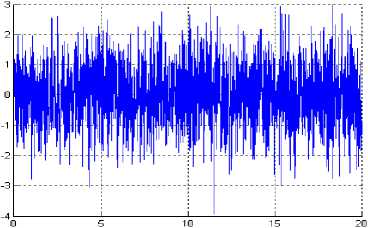
Fig. 7: Uniform Random White Noise

Case 3: External Disturbance is Lugre friction. The LuGre model is a dynamic friction model presented in [33]. Lugre Fiction can be modeled mathematically as in Eqs. (23-25) given below:

■

̇ =V

^{| и}- | д ( V )

F =    + (Jv ̇+y₂V           (24)

д ( V )= f_c +( Fs - F_c )exp( )²        (25)

where z is average bristle deflection, ^o is stiffness of bristles, ^1 is bristle damping coefficient, (J₂ is viscous damping coefficient, v is relative velocity between moving parts, F_c is coulomb coefficient, F_s is static coefficient, ^s is striberk velocity. Constants parameters for the Lugre friction are taken as

^0 = ․6, ^vs = ․04,

F = ․01, F₍ = 10

Case 4: External disturbance is combination of white noise and Legru friction.

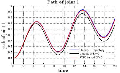
Fig. 8: Trajectory tracked: Joint 1 in Case 4.

Fig. 9: Trajectory tracked: Joint 2 in Case 4.

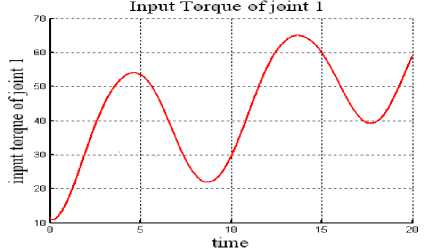
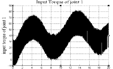
Fig. 13: Control Input Torque: Joint 1 of PSO tuned SMC.

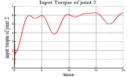
Fig. 14: Control Input Torque: Joint 2 of PSO tuned SMC.

time

Fig. 11: Control Input Torque: Joint 1 of classical SMC.

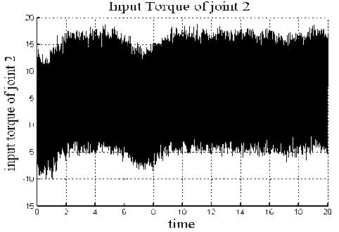
Fig. 12: Control Input Torque: Joint 2 of classical SMC.

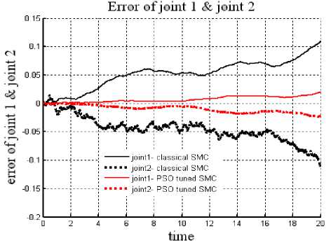
It has been observed from the table 2 that when compared with the classical SMC, mse of the tracking error for the PSO tuned SMC is lesser in the cases i.e. with and without uncertainties.

• VI.    Conclusions

This paper proposes an improved PSO algorithm for improving the control performance of the conventional controllers naming PID and SMC by finding the optimal values of the constant control parameters used in these control techniques. It has been observed from the results that this hybrid of modified PSO with classical controllers (PID and SMC) gives significantly improved for motion control problem of a manipulator. Trajectory tracking performance of manipulator improvising with the proposed controllers. It can also be observed that the mse error of system with the proposed hybrid controllers reduces even in presence of uncertainties too. Hence, it can be said that the robustness of the system controllers has increased. It can be concluded that the proposed control scheme is quite efficient.

Table 2. MSE of tracking error for classical and PSO tuned SMC: Case 1-4.

Controller	Classical SMC		PSO tuned SMC
Case	Joint 1	Joint 2	Joint 1	Joint 2
I (no disturbance)	1.45E-04	2.08E-04	2.86E-05	2.46E-05
II (noise)	1.53E-04	2.02E-04	4.79E-06	3.54E-06
III (Legru friction)	2.74E-04	3.01E-04	2.30E-04	2.97E-04
IV (noise+Legru friction)	0.0035	0.0028	3.42E-05	7.89E-05