Improving plot-level growing stock volume estimation using machine learning and remote sensing data fusion

Forests are among the highly valuable natural resources, along with freshwater sources, mineral deposits, and fertile soil. Exploration of environmental variables supports ecologically sustainable development of regions and a significant level of biodiversity [1]. Modern silviculture involves advanced methods to collect and actualize inventory data across vast territories [2]. This data are used for forest management decisionmaking based on timber product content and quality measurement and can also be utilized to prevent forest degradation caused by natural and anthropogenic reasons. Forests are usually described by species distribution, tree age, and height assessed through ground-based observations and measurements [3]. However, while forest species, age, and height can be considered intermediate parameters for further analysis, timber stock or growing stock volume (GSV) is the ultimate parameter for forestry management and decision-making. Therefore, a number of studies are currently focused on estimating this characteristic.

Recently, remote sensing observations have become an advanced tool to facilitate forestry research. Depending on the scope and requirements of the investigation, scholars can consider data derived from satellite observations and unmanned aerial vehicles

(UAVs). UAVs have higher spatial resolution and are capable of capturing fine-grained details compared to satellite observations. It has already been shown that UAV-based measurements can be effectively integrated into pipelines for estimating forest characteristics [4, 5]. However, the main disadvantages are associated with the limited territories that can be covered by UAVs and the cost of sensing equipment. On the other hand, satellite-derived images are intended to provide information about vast territories that can be further used for forestry studies. High-resolution satellite observations are provided by satellite constellations such as WorldView, QuickBird, GeoEye, IKONOS distributed by DigitalGlobe (USA). Currently, the China National Space Administration (CNSA) has also launched the high-resolution Gaofen satellite mission that brings new opportunities in geospatial research [6]. Roscosmos (the state corporation of the Russian Federation responsible for space flights) also provides high-resolution satellite observations such as imagery from Resurs-P space system. The main limitation for the high-resolution remote sensing data application in forestry studies is their high cost. Medium-resolution satellite data are freely available and have a high frequency of observations for satellite constellations such as the Sentinel mission developed by the European Space Agency or the Landsat mission hosted by the USGS’s Earth Resources

Observation and Science (EROS) Center. The wide range of spectral bands (13 bands) of the Sentinel-2 satellite supports accurate analysis of vegetation cover and can be used for estimating forest characteristics with a spatial resolution up to 10 meters. Due to sufficient spatial resolution and short revisit time (5 days), it meets practical demands in various environmental tasks [7]. For instance, these data successfully assist in forest growing stock volume estimation in the Russian Southern Taiga region [8]. In addition to utilizing a single data source, remote sensing data fusion is a crucial topic for investigation that can enhance the quality of environmental analysis [9].

Machine learning algorithms are successfully applied for remote sensing data processing in various environmental and geospatial tasks [10]. They enable faster data analysis on a global and local scale. In forestry research, machine learning algorithms are utilized to estimate characteristics such as forest species, tree canopy height, forest age, volume, and more. The forest structure can be predicted using LiDAR measurements and machine learning algorithms, as demonstrated in [11]. A number of studies explore the application of classical machine learning algorithms like Random Forest, Gradient Boosting, Support Vector Machines, and others to estimate forest characteristics through satellite data [12, 13, 14]. Deep learning methods are also employed in the pipeline for extracting forest parameters [15, 16]. Typically, reference forestry data used to train machine learning models are derived from individual stand-based measurements [17, 13]. Individual stands are considered as an indivisible unit of study, despite being typically non-homogeneous [18]. This means that each individual stand may contain trees with varying properties, and the dominant species, the average age, height, and volume are determined within the stand. The maximum stand area is dependent on the level of taxation and can be up to 20 hectares. This data is suitable for specific tasks and can be utilized for mapping large regions [19]. However, more precise taxation data is collected for sample plots (referred to as plot-level taxation) [20]. Sample plots have a smaller area and provide more homogeneous measurements for multiple trees. Due to the labor-intensive nature of data collection, fewer studies have utilized such data for machine learning development [21, 22]. For the Russian arctic, plot-level data with 33 field plots were applied in [23] to estimate the growing stock volume.

In this study, our focus is on developing an effective pipeline for precise forest growing stock volume mapping based on freely-available medium-resolution satellite data. As the reference data, we chose forest sample plots to maintain accurate field-based measurements. Each plot has a diameter of 9m, and the entire dataset comprises more than 600 individual sample plots. The dataset was generated using medium-resolution multispectral satellite imagery from Sentinel-2. In addition to the original spectral bands, we also incorporated auxiliary data to extract additional significant information about forest cover. We conducted experiments with vegetation indices computed from spectral bands and a canopy height model (CHM) derived from airborne laser scanning. Several techniques were explored to create training samples by aggregating satellite observations from different summer periods to enhance the robustness of the solution. The proposed approach was validated in the Perm region of eastern European Russia using inventory data collected in 2022. The main contributions of the study are the following:

• •    A unique dataset comprising several groups of features was collected and analyzed;

• •    We proposed and validated two approaches for growing stock volume estimation using sample plots measurements as the reference data;

• •    We compared several machine learning algorithms.

1.    Methods and data 1.1.    Inventory field-based measurements

The study area is located within the territory of Kolvinsky Forestry in the northern part of the Perm Krai, on the border with the Komi Republic. The territory of the forestry belongs to the Middle Ural taiga forest region. Based on the species and age characteristics, the area can be conventionally divided into two parts. The first (central and southern) part consists of secondary forests formed in places of concentrated deforestation during the 1970s-1990s. The second (northern) part of the plot represents relatively undisturbed forest areas, where human impact on the natural environment is virtually absent.

In our study, we utilize sample plots, which are defined as indivisible units of forested areas, each comprising small forested territories where ground-based measurements were conducted.The sample plots were established covering both parts of the site and were positioned within a two-kilometer zone relative to existing roads and rivers, along which it was feasible to organize the movement of groups of engineer-assessors. These plots consisted of circular plots with a constant radius of 9 meters and were grouped into clusters of 9, arranged in a 3×3 square configuration (Fig. 1). The central number denotes the cluster number. All measurements of the plots within each cluster are conducted by the same forestry brigade.

Within the boundaries of each sample plot, measurements of tree trunk diameters were taken at a height of 1.3 meters above the root collar of trees with diameters greater than 6 centimeters. The species of the tree, its vitality (alive or dead), and the characteristics of stem development (presence of branching, curvature, absence of tops, etc.) were recorded. Additionally, for each species, the height and age of three model (average diameter-wise) trees were measured.

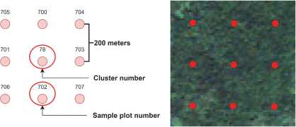
Fig. 1. Cluster scheme used in the forest inventory in the Kolvinsky forestry district of the Perm Krai and an example of Sentinel-2 image aligned with the sample plots

Based on the measurement results for each sample plot, the average taxation characteristics of the plantings were calculated, including volume (cubic meters per hectare), average height (meters), average diameter (centimeters), average age (years), and sum of sectional areas (square meters per hectare) both overall and for each species component within the sample. All measurement data, comprising 693 data points, were stored in CSV format.

• 1.2.    Remote sensing data acquisition and processing

In the present study, multispectral imagery from Sentinel-2 L2A was selected as the primary data source (Fig. 2), accessed through the Google Earth Engine service, which provides access to an extensive collection of geospatial data [24]. The satellite images possess channel resolutions ranging from 10 meters to 60 meters per pixel. To mitigate potential distortions caused by atmospheric phenomena and cloud cover, median values of the imagery acquired during clear, summer periods were chosen for analysis in this study. This approach minimizes the influence of factors unrelated to the condition of forested areas, ensuring more accurate and consistent data for analysis [25].

Each image obtained from Sentinel-2 L2A comprises 13 channels, providing information on various land surface characteristics (Table 1). For the purposes of this study, we chose 10 channels (B02-B8A, B11, and B12) with the spatial resolution from 10 to 20 meters per pixel.

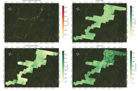
Fig. 2. RGB composite of the Sentinel-2 image with sample plots; Canopy height models; Digital elevation models; Forest age map

Tab. 1. Description of Sentinel-2 bands

Band	Description	Wavelength	Pixel Size
		(nm)	(m)
B01	Coastal aerosol	443.9	60
B02	Blue	496.6	10
B03	Green	560	10
B04	Red	664.5	10
B05	Red Edge 1	703.9	20
B06	Red Edge 2	740.2	20
B07	Red Edge 3	782.5	20
B08	NIR	835.1	10
B8A	Red Edge 4	864.8	20
B09	Water vapor	945	60
B10	SWIR Cirrus	1375	60
B11	SWIR 1	1613.7	20
B12	SWIR 2	2202.4	20

Furthermore, for vegetation analysis on the land cover, vegetation indices such as NDVI and EVI were computed [26].

NDVI reflects differences in light absorption by various vegetation types and is calculated using the formula:

NDVI =

NIR - Red

NIR + Red ,

where:

NIR is the near-infrared reflectance, Red is the red reflectance.

EVI is utilized to assess plant health and is calculated using the formula:

EVI = 2.5 x

______ NIR - Red ______

NIR + 6 x Red - 7.5 x Blue + 1

where:

NIR is the near-infrared reflectance,

Red is the red reflectance,

Blue is the Blue reflectance.

The laser scanning data were collected in 2022. Flights were conducted in the first half of June and the second half of August. The June survey employed a Lieca

ALS 80 scanner, while the August survey utilized a Lieca ALS 60. The scanning data had a density of no less than 3 points per square meter. The final probable accuracy of determining the planned position of laser reflection point was up to 0.25 meters horizontally and up to 0.09 meters vertically. Canopy Height Model (CHM) was derived representing numerical values of vegetation height. Additionally, Digital Elevation Model (DEM) was generated from satellite data, representing the elevation of the Earth’s surface above sea level [27]. These data are depicted in Fig. 2, with their corresponding distributions in Fig. 3. All these images were downsampled to a resolution of 10 meters per pixel using the nearest neighbor algorithm to match with Sentinel-2 image. Furthermore, data obtained using machine learning algorithms for estimating tree age were included in the study, allowing for the consideration of growth dynamics and development of forest stands in the study region [28]. This auxiliary data facilitated a more comprehensive understanding of the state of forest ecosystems and the factors influencing their development.

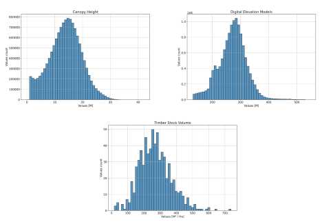
Fig. 3. The distribution of the canopy height model (CHM), the digital elevation model (DEM), and the timber stock within the study area

• 1.3.    Problem definition

The goal of the study is to develop an effective machine learning-based approach for growing stock volume (GSV) estimation using satellite data and auxiliary spatial characteristics. The GSV denotes the total volume of all living tree stems, excluding branches and including barks, in an area of interest or unit area such as a hectare [23]. We focus on the sample plot inventory data due to their higher reliability and precision than individual stand measurements. One of the major issues in solving this task is associated with data selection, preprocessing, and further integration into an ML model. The combination of these parts is intended to provide a solid methodology for timber stock estimation for vast territories using available data. In terms of machine learning, we define the task as a regression problem with the target timber stock values. We propose to consider two approaches for creating objects representing each sample plot for further ML algorithm training. The first approach involves processing a single “central” pixel for each sample plot, while the second approach relies on a set of pixels that lie within the sample plot. Let’s entitle the first approach point-based and the second approach polygon-based. In the first case, an object can be described by a set of spectral values extracted from the satellite image belonging to a single pixel. These features can be supplemented by vegetation indices described in the previous section, as well as auxiliary data such as CHM and DEM. It is worth noting that the pixel size of 10×10 meters lies entirely within the sample plot with a radius of 9 meters. In the polygonbased approach, each sample plot can be described by a set of pixels with spectral features, indices, CHM, DEM, and forest age. The total number of pixels lying within the sample plot or intersecting its boundary can be 4, 6, or 9 pixels depending on the shift of plot boundaries and satellite image. To maintain a constant number of features for these cases (4, 6, or 9 pixels), instead of directly using all pixels overlaying the sample plot, we aggregate them and compute statistics for each initial feature. We analyzed the importance of several groups of features and assessed the applicability of the approach in cases where CHM and DEM data are absent.

To assess the feasibility and advantages of these approaches, we consider three machine learning algorithms, including classical machine learning and deep learning.

During inference time, the developed models can be easily applied to new territories using a desired group of features, including Sentinel-2, CHM, DEM, forest age, or all of them. As an additional feature, we also considered sample plot coordinates. This data can be integrated in practical cases when a set of sample plots are available for forestry and the goal is to map the entire territory. However, if the inference is conducted for territories located outside of the base forestry, longitude and latitude features should be excluded from consideration.

A more detailed description of each step of the study is presented below.

• 1.4.    Experimental workflow

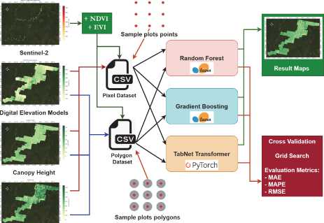
Data preprocessing was performed using two approaches: point-based and polygon-based. In the first approach, each central point represented in CSV format was associated with the corresponding pixel in the Sentinel-2 image, as well as CHM and DEM data. This operation facilitated the linkage of point attribute, such as timber stock volume (V), with corresponding geospatial data. Subsequently, vegetation indices reflecting the vegetation status in the analyzed area were computed. The resulting dataset was then written to a CSV file.

In the second approach, based on the data from the CSV file, the radius of each point was computed, serving as the basis for polygon construction. These polygons were then intersected with Sentinel-2, CHM, and DEM images to link the polygons with corresponding geospatial data. Similar vegetation index computations were then conducted. Statistical characteristics, including minimum and maximum values, sum, standard deviation, mean, median, and variance, were calculated based on the obtained data. These results were also recorded in CSV format.

Also for all images, pixels intersecting with the cloud mask were removed.

The next stage involved applying three different types of models: Random Forest (RF), Gradient Boosting (GB), and the TabNet transformer model. To evaluate the effectiveness of the proposed models, cross-validation techniques were employed in combination with quality metrics. These metrics aid in determining the accuracy of the models and enable the comparison of their performance based on various characteristics of the predicted data. By applying cross-validation, we ensure a more objective assessment of model quality, considering data variations and reducing the likelihood of overfitting.

Forest Age

Fig. 4. Experimental pipeline. We utilize several remote sensing data sources and field-based measurements to create the dataset. Then, three machine learning algorithms are trained to produce the ultimate geospatial maps

For the analysis of forest resources, sample plot data from the forest inventory table were employed, containing information on growing stock volume, serving as the target variable (V). Moreover, the analysis incorporated images containing information on CHM and DEM which provided additional characteristics for the objects under analysis.

Additionally, hypotheses were tested involving the use of different feature combinations for model training. This process aimed at identifying the most informative features contributing to the enhancement of model prediction quality. All combinations of features were divided into several groups:

• 1.    Sentinel-2 bands, Vegetation indices

• 2.    Sentinel-2 bands, Vegetation indices, Coordinates

• 3.    Sentinel-2 bands, Vegetation indices, CHM

• 4.    Sentinel-2 bands, Vegetation indices, DEM

• 5.    Sentinel-2 bands, Vegetation indices, CHM, DEM

• 6.   Sentinel-2 bands, Vegetation indices, CHM,

• 7.   Sentinel-2 bands, Vegetation indices, CHM,

DEM, Coordinates

DEM, Coordinates, Age

• 1.5.    Machine learning algorithms

In this study, a set of three machine learning models was selected to address the regression task. The first two models, based on decision trees, are RF and GB. The primary concept of RF involves dividing the training data into samples, with each tree trained on its sample, followed by averaging the predictions of individual trees to obtain the final result [29]. In Gradient Boosting, each subsequent tree aims to correct the errors of the previous ones, thereby gradually improving the model’s quality [30]. The scikit-learn (sklearn) implementation was chosen for these models [31].

Additionally, a transformer model specialized in tabular data analysis, known as TabNet [32], was tested and PyTorch implementation was used [33]. The TabNet algorithm employs a sequential attention mechanism to select features based on which decisions are made at each step, thereby enhancing interpretability and training efficiency by focusing computational resources on the most significant features. This is achieved through masking for soft feature selection, rendering the algorithm more parametrically efficient.

The parameter tuning process for the models was conducted using the grid search method, allowing systematic evaluation of model performance for various parameter combinations and selecting the optimal ones. The following are the models and grids used for parameter optimization:

Random Forest:

• •    n_estimators (number of trees): 50, 100, 200, 400, 600

• •    max_features (number of features in searching for the best split): auto, sqrt, log2

• •    max_depth (maximum depth of the tree): 3, 4, 5, 6, 7, 8

• •    criterion (function evaluating the quality of a split): absolute_error, squared_error, poisson, friedman_mse

Gradient Boosting:

• •    n_estimators (number of trees): 50, 100, 200, 400, 600

• •    max_features (number of features in searching for the best split): auto, sqrt, log2

• •    max_depth (maximum depth of the tree): 3, 4, 5, 6, 7, 8

• •    learning_rate (set the contribution of the tree): 0.01, 0.1, 0.5

• •    loss (optimization function): ls, lad, huber, quantile

TabNet:

• •    n_d (width of the decision prediction layer): 8, 16, 32

• •    n_a (width of the attention embedding for each mask): 8, 16, 32

• •    n_steps (number of steps in the architecture): 3, 5, 10

To select the optimal model parameters and obtain reliable metric evaluations, we employed cross-validation using 5 folds. Within this approach, the entire original dataset was partitioned into five parts, where one part was utilized as the test dataset, and the remaining four served as training data for the model. Subsequently, model performance was evaluated. During each subsequent iteration, a different fold was chosen for testing, and the other four folds were used for model training, repeating the process for all folds. Ultimately, the metrics obtained after five iterations were averaged to obtain a generalized assessment of model performance.

• 1.6.    Models performance evaluation

To assess the effectiveness of models, three main metrics were utilized: Mean Absolute Error (MAE), Mean Absolute Percentage Error (MAPE), and Root Mean Square Error (RMSE). Each of these metrics possesses its unique characteristics, providing information about the accuracy of model predictions.

MAE represents a readily interpretable metric; however, it is insensitive to outliers in the data. This implies that even significant errors in predictions do not heavily impact this metric.

1 ⁿ

MAE =-L । y< - У‘ I, n =1

where:

n is the number of observations, y is the observed value, y ˆ is the predicted value.

RMSE is sensitive to large errors in the data. It assigns a higher weight to significant errors, making it useful in detecting and highlighting potential outliers.

n

Rmse = a -L( y - y) ² , n i =1

where:

n is the number of observations, y i is the observed value, y ˆ _i is the predicted value.

MAPE serves as a useful tool for measuring the percentage error of forecasts. However, it should be noted that this metric may encounter issues when actual values are close to zero or equal to zero.

n

MAPE = -У ni=1

y, - y y i

x l00%

Where:

n is the number of observations, y is the observed value, yˆ is the predicted value.

2.    Results and discussion

In this study, we aim to develop a machine learningbased approach to map growing stock volume through remote sensing data. Several setups were examined for a deeper understanding of the connections between spectral characteristics and the reference inventory measurements. Point and Polygon-based approaches were proposed to consider a single Sentinel-2 pixel or a set of pixels related to each sample plot. Three machine learning algorithms, RF, GB, and TabNet, were selected to conduct the study. The achieved results for the Point-based approach are presented in Table 2 and for the Polygon-based are shown in Table 3. For each machine learning algorithm, several groups of features were employed. We considered Sentinel-2 bands with vegetation indices separately as a baseline solution for both Pixel and Polygon-based approaches. For this data, the MAE varies from 71 m3/ha to 74 m3/ha for the Point-based approach and 73 m3/ha for the Polygon-based approach depending on the machine learning algorithm. Further experiments with auxiliary input features allowed us to adjust the initial results. The best results were achieved for the combination of all available geospatial features. For the Point-based approach, the lowest MAPE equals 31.7 % using the RF algorithm. For the Polygon-based approach, the lowest MAPE is achieved by the GB algorithm at 30.5%. While all algorithms show comparable results for the initial feature set, RF and GB algorithms perform better than the TabNet algorithm when new features are added. In further study, additional investigation on deep learning algorithms for tabular data should be conducted.

In forestry applications, it is vital to separate two cases: when UAV-based measurements are available and when only satellite-based observations are provided for the study. Therefore, we explore Sentinel-2 data with freely available geospatial features apart from the UAV data. DEM data can be employed to improve prediction quality and reduce the MAE on average to 2 m3/ha or 2% for the MAPE metric. Moreover, we examined the contribution of coordinate information as an additional feature. Although this data can be used only in cases of mapping the same study territory where the sample plots are located, it allows us to reduce the MAPE metric on average to 2.7% compared to the baseline solution. For several models, improvements in the MAPE metric are larger than 5%.

CHM derived from LiDAR measurements serves as an important input feature to estimate timber stock. It leads to the most significant improvements (reduces the MAPE by 8%) for the RF and GB models in the Polygon-based setup. Therefore, the availability of LiDAR data is crucial for precision silviculture studies. In some cases, this data can be substituted by artificially generated canopy height through remote sensing data and deep learning algorithms [34].

Tab. 2. Prediction results for the Point-based approach on the test data

Model	Sentinel	CHM	DEM	lon, lat	age	MAE	MAPE	RMSE
Random	+	-	-	-	-	74,726	0,396	95,937
Forest	+	-	-	+	-	69,399	0,356	90,032
	+	+	-	-	-	66,998	0,345	87,635
	+	-	+	-	-	73,089	0,385	94,001
	+	+	+	-	-	66,024	0,338	86,384
	+	+	+	+	-	64,077	0,317	83,98
	+	+	+	+	+	64,161	0,319	84,129
Gradient	+	-	-	-	-	74,33	0,392	95,844
Boosting	+	-	-	+	-	69,988	0,355	90,426
	+	+	-	-	-	67,579	0,346	88,088
	+	-	+	-	-	72,273	0,377	93,182
	+	+	+	-	-	67,768	0,34	88,192
	+	+	+	+	-	65,262	0,322	85,19
	+	+	+	+	+	65,197	0,321	85,131
TabNet	+	-	-	-	-	71,649	0,38	92,901
	+	-	-	+	-	70,727	0,371	92,388
	+	+	-	-	-	69,922	0,362	90,657
	+	-	+	-	-	70,268	0,365	90,926
	+	+	+	-	-	69,93	0,363	90,412
	+	+	+	+	-	69,413	0,362	89,381
	+	+	+	+	+	68,999	0,36	89,049

Tab. 3. Prediction results for the Polygon-based approach on the test data

Model	Sentinel	CHM	DEM	lon, lat	age	MAE	MAPE	RMSE
Random	+	-	-	-	-	73,868	0,382	95,173
Forest	+	-	-	+	-	71,05	0,361	92,171
	+	+	-	-	-	65,171	0,325	84,982
	+	-	+	-	-	71,19	0,363	92,192
	+	+	+	-	-	63,971	0,32	84,316
	+	+	+	+	-	63,447	0,31	83,399
	+	+	+	+	+	63,813	0,31	83,622
Gradient	+	-	-	-	-	73,234	0,376	94,641
Boostin g	+	-	-	+	-	70,318	0,351	91,483
	+	+	-	-	-	65,943	0,323	85,839
	+	-	+	-	-	71,331	0,357	92,487
	+	+	+	-	-	65,122	0,317	85,206
	+	+	+	+	-	63,986	0,308	84,244
	+	+	+	+	+	63,89	0,305	84,066
TabNet	+	-	-	-	-	73.422	0.387	94.852
	+	-	-	+	-	73.62	0.382	95.549
	+	+	-	-	-	71.243	0.364	92.337
	+	-	+	-	-	71.938	0.367	93.119
	+	+	+	-	-	70.989	0.35	92.074
	+	+	+	+	-	70.152	0.344	91.077
	+	+	+	+	+	69.737	0.342	90.578

For the point-based approach optimal parameter setting was achieved for the combination of features: Sentinel bands, Vegetation indices, CHM, DEM, Coordinates and using model parameters: n_estimators = 600, max_features = sqrt, criterion = poisson, and max_depth = 8. But for the polygon-based approach we achieved peak performance using Gradient Boosting models with combination of features: Sentinel bands, Vegetation indices, CHM, DEM, Coordinates, Age and parameters: n_estimators = 400, max_features = sqrt, max_depth =4, learning_rate = 0.01, and loss = huber.

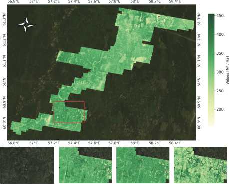
Visual results of these models are presented in Fig. 5 and Fig. 6. The obtained maps can be further utilized in comprehensive analysis alongside data collected from other environmental sources, such as maps with different spatial resolutions or measurements from individual stands. Additionally, in visual analysis, we can observe that some models tend to overestimate the predicted values compared to others. However, the general spatial patterns remain similar across all models observed. These generated maps can be valuable in forestry studies covering extensive territories.

The age measurements derived from the earlier study allows us to improve the results slightly in some machine learning setups.

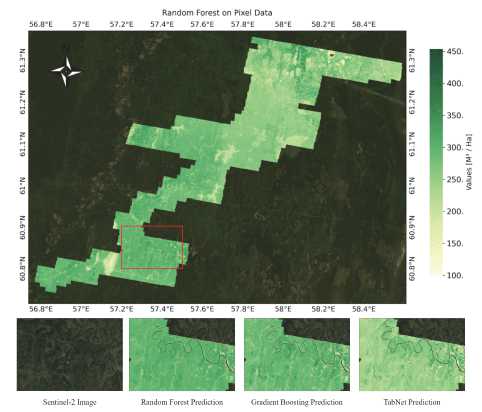
Fig. 5. Visual results of the top-performing model Random Forest trained on point-based approach data, under the optimal combination of parameters including Sentinel-2 bands, Vegetation indices, CHM, DEM, and Coordinates, are presented. Additionally, a comparison with alternative models using the same dataset is provided

Gradient Boosting on Polygon Data

Sentinel-2 Image             Random Forest Prediction Gradient Boosting Prediction           TabNet Prediction

Fig. 6. Visual results of the top-performing model Gradient Boosting trained on polygon-based approach data, under the optimal combination of parameters including Sentinel-2 bands, Vegetation indices, CHM, DEM, Coordinates, and Age, are presented. Additionally, a comparison with alternative models using the same dataset is provided

The direct comparison with other studies is difficult to conduct due to non-publicly available datasets collected for each study. The data varies in terms of studied forest species, tree age, and environmental conditions. However, our achieved results are generally comparable with metrics performed in previous studies. For instance, in [35], the best RMSE metric equals 65.03 m3 /ha for the RF model for Chinese forests, while in our case the best RMSE is 83.39 m3 /ha. In [21], using a combination of unmanned aerial systems (UASs), terrestrial laser scanning (TLS), and synthetic aperture radar (SAR) from satellites, they achieved RMSE values ranging from 66.87 m3 /ha to 80.12 m3 /ha for plot-level stem volume measurements in Japanese forests. However, these data sources require additional equipment to conduct the study. Overall, the achieved results show high potential for further usage in environmental studies and silviculture management.

Conclusion

Machine learning (ML) algorithms prove to be a powerful tool in geospatial monitoring and analysis using remote sensing observations. However, forestry tasks require developing highly specialized approaches that take into account the origin of the forest inventory data. Although a common choice of such data is individual stands, more precise field-based measurements are associated with sample plots. The proposed solution focuses on the application of medium-resolution (10 m per pixel) satellite data to estimate growing stock volume (GSV) in forests of eastern European Russia. We examined different feature spaces with original spectral bands and vegetation indices based on them. In addition to satellite-derived data, we assessed the importance of the canopy height model (CHM) from airborne laser scanning for timber stock estimation. Among the considered ML algorithms, Gradient Boosting shows the highest performance. As a result, the solution can be used for geospatial map creation for vast and remote territories, reducing the cost and time for field-based measurements.

Acknowledgements

The work was supported by the Russian Science Foundation (Project No. 23-71-01122).