Information dynamic analysis and measure of quantum algorithm's computational intelligence

Author: Barchatova Irina, Degli Antonio Giovanni, Ulyanov Sergey
Journal: Сетевое научное издание «Системный анализ в науке и образовании» @journal-sanse
Article in issue: 3, 2014.
Free access
Information dynamic analysis of main quantum algorithms is described. The qualitative analysis of quantum information is introduced. Measure of quantum algorithm’s computational intelligence is discussed.
Information analysis, information measure of quantum algorithm's computational intelligence, qualitative analysis of efficiency simulations
Short address: https://sciup.org/14123243
IDR: 14123243
Информационный динамический анализ и меры интеллектуальности квантовых алгоритмов
Представлен информационный анализ основных квантовых алгоритмов и качественный анализ квантовой информации. Рассмотрено меры вычислительного интеллекта квантовых алгоритмов.
Text of the scientific article Information dynamic analysis and measure of quantum algorithm's computational intelligence
Introduction: Information analysis axioms of quantum algorithm dynamic evolution
The qualitative analysis of quantum information is described in [1 – 5]. Any computation (both classical and quantum) is formally identical to a communication in time. By considering quantum computation as a communication process, it is possible to relate its efficiency to its classical communication capacity. At time t = 0 , the programmer ( M ) sets the computer to accomplish any one of several possible tasks. Each of these tasks can be regarded as embodying a different message. Another programmer ( C ) can obtain this message by looking at the output of the computer when the computation is finished at time t = T . Computation based on quantum principles allows for more efficient algorithms for solving certain problems than algorithms based on pure classical principles.
Remark 1 . The sender conveys the maximum information when all the message states have equal a priori probability (which also maximizes the channel capacity). In that case the mutual information (channel capacity) at the end of the computation is log N .
The communication capacity gives an index of efficiency of a quantum computation [6]:
A necessary target of a quantum computation is to achieve the maximum possible communication capacity consistent with given initial states of the quantum computing .
Let us consider any peculiarities of information axioms and information capability of quantum computing as the dynamic evolution of quantum algorithms (QAs). If one breaks down the general unitary transformation U of a QA into a number of successive unitary blocks, then the maximum capacity may be achieved only after the number of applications of the blocks. In each of the smaller unitary blocks, the mutual information between the M and the C registers (i.e., the communication capacity) increases by a certain amount. When its total value reaches the maximum possible value consistent with a given initial state of the quantum computing, the computation is regarded as being complete (see, in details [6, 7]). The classical capacity of a quantum communication channel is connected with the efficiency of quantum computing using entropic arguments. This formalism allows us to derive lower bounds on the computational complexity of QA’s in the most general context. The following qualitative axiomatic descriptions of dynamic evolution of information flow in a QA are provided [8, 9]:
|
N |
Axiomatic Rules |
|
1 |
The information amount (information content) of a successful result increases while the QA is in execution |
|
2 |
The quantity of information becomes the fitness function for the recognition of successful results on intelligent states and introduces the measures of accuracy and reliability (robustness) for successful results. |
|
In this case the principle of Minimum of Classical / Quantum Entropy (MCQE) corresponds to recognition of successful results on intelligent states of the QA computation |
|
|
3 |
If the classical entropy of the output vector is small, then the degree of order for this output state relatively larger, and the output of measurement process on intelligent states of a QA gives the necessary information to solve the initial problem with success |
Remark 2 . These three information axioms mean that the algorithm can automatically guarantee convergence of information amount to a desired precision with a minimum decision making risk. This is used to provide robust and stable results for fault-tolerant quantum computation. Main information measures in classical and quantum domains are shown in Tables 1 and 2.
Table 1. Typical measures of information amount
|
Title |
Classical ( Cl ) |
Quantum ( Q ) |
||
|
Fisher |
2 |
rrz p x ) )12 Tr E ( q d x F Q ( x ) = J L\am , tl d q Tr ( E ( q ) p ( x ) ) |
||
|
F a ( x )=f 1 |
д P ( q x ) d x |
d q |
||
|
J p ( q x ) |
||||
|
Boltzman - Shannon u von Neumann |
S Sh =- Z p i |
i ln pi |
Sv N = - Tr ( p ln p ) |
|
|
Relative Information - Kullback - Leibler |
I C ( p : q ) = -] |
pi ln q i i pi |
I Q ( p : e r ) = - Tr | p ln p | V e 7 |
|
|
Renyi |
s ( Cl ) R = l q 1 - q |
W Z p q V i =1 7 |
ln Tr ( p q) S ( Q ) R = L V /J q 1 - q |
|
|
Havrda & Charvat - Daròczy ( Tsallis ) |
W i - Z p q ( Cl ) T _ I i =1 7 q 1 - q |
1 - Tr p q S ( Q ) T = \------- q 1 - q |
||
Table 2. Relations between different typical measures of information amounts
-
1. Shannon and von Neumann Entropy Relation SvVN < S Sh For Diagonal Density Matrix: p = p and S vN = S Sh
-
2. Tsallis q-Entropy and Shannon Entropy Relation
-
3. Tsallis q-Entropy and Renyi Entropy Relation
s (°) R =
i - q
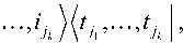
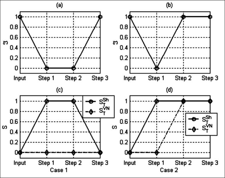
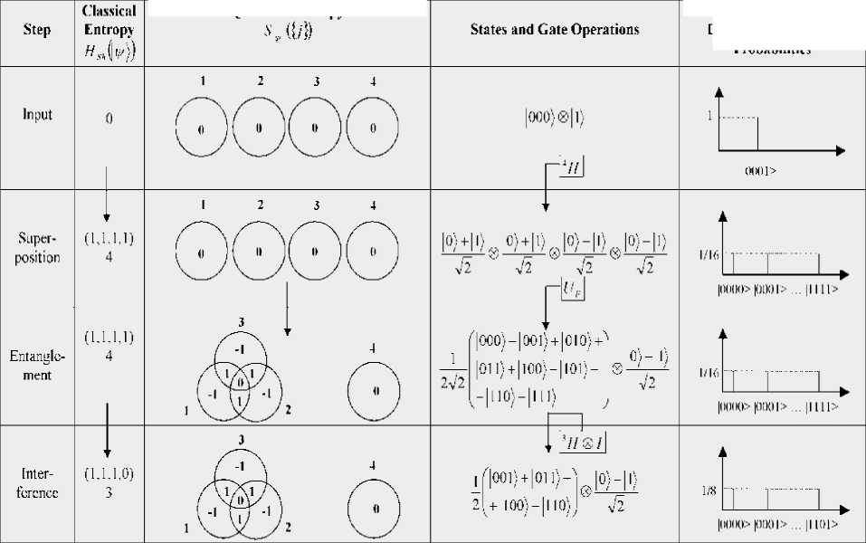
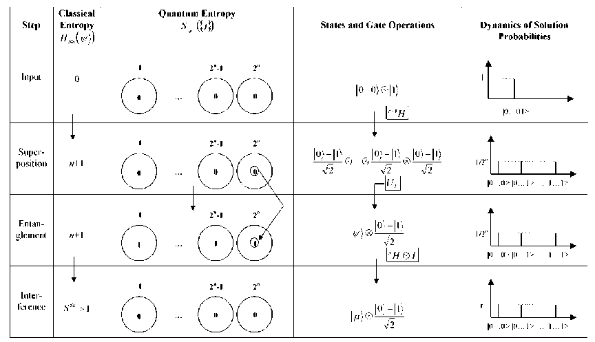
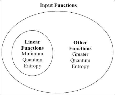
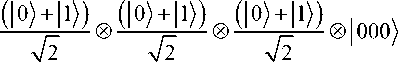
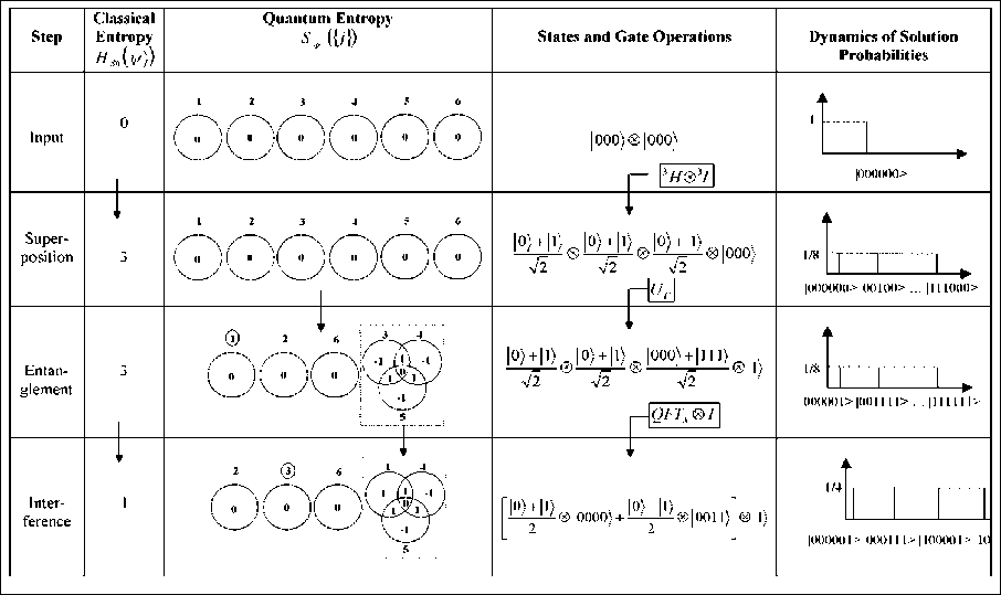
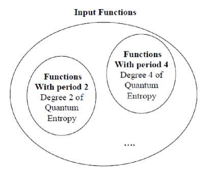
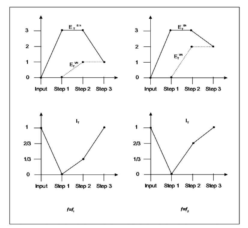
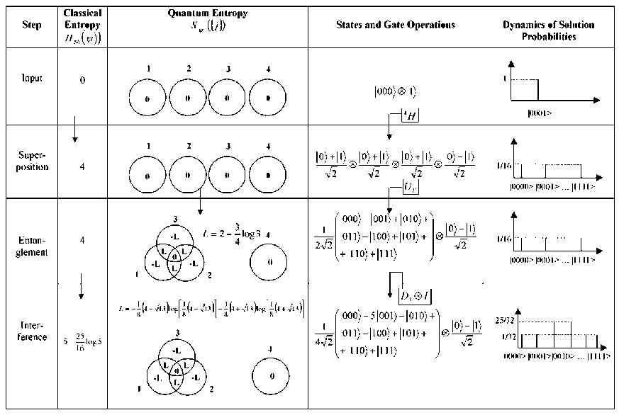
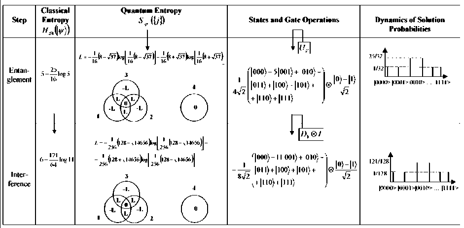
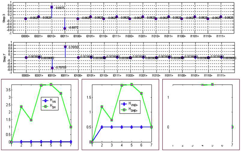
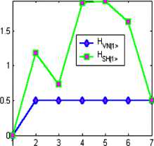
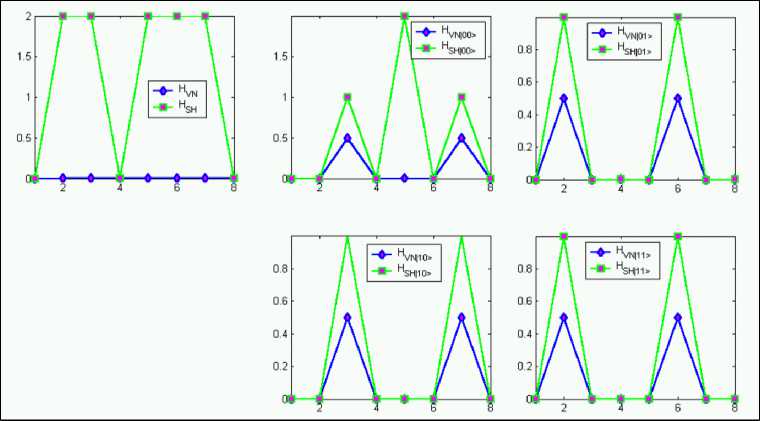
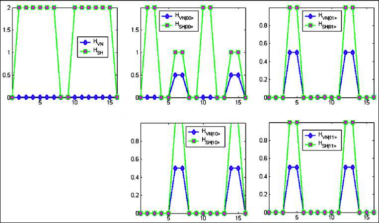
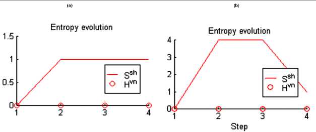
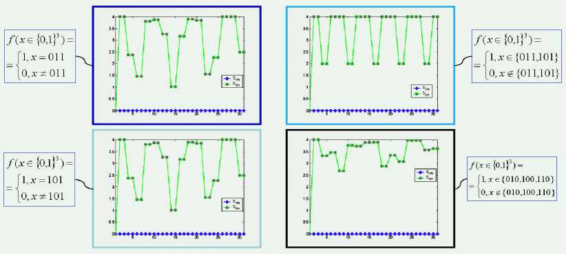
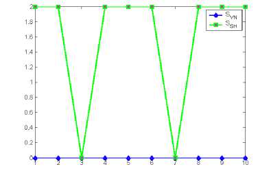
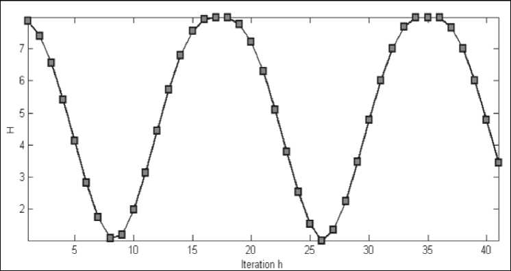
W limS Remark 3. Five main information-based approaches in optimal design of QA’s computation can be used: 1) the maximum entropy (ME) principle; 2) minimum Fisher information (MFI) principle; 3) principle of extreme physical information (EPI); 4) principle of maximum of mutual information (MMI) between computational and measurement dynamic evolution (computational and memory registers) of QA’s; and 5) principle of maximal intelligence of QA’s based on minimum of difference between classical and quantum entropies in intelligent states of successful results. The first three principles (ME, MFI, and EPI) are based on the physical laws and may be derived through variation on appropriate Lagrangian’s and includes in last two principles according to relations between the classical and quantum entropies, and mutual information amount. The main properties of quantum information and entropy measures, and interrelations between information amounts (classical and quantum measures) are described in [8]. Remark 5. The EPI principle differs significantly from the EM approach or the MFI approach: (1) In its aims (establishing on ontology in EPI and eliciting the laws of physics from a consideration of the flow of information in the measurement process, vs subjectively estimating the laws in ME or MFI); (2) in its reason for extremization (conservation of information in EPI, vs arbitrary, subjective and sometimes inappropriate choice of «maximum smoothness» in ME and MFI); (3) how «constraints» are chosen (via the invariance of information to a symmetry operation principle in EPI vs arbitrary subjective choice in ME or MFI); and (4) in its solutions (to a differential equation in EPI and MFI, vs a solution, always in the form of an exponential of a function, in ME). Only EPI applies broadly to all of physics principles1,2,34,5. Information intelligent measure of QA’s (principle 5) The information intelligent measure of QA as IT (V1)) of the state jV’} with respect to the qubits in T and to the basis B = {| i^ ® • • • ® | in )} is [8, 9] /I n sS*^--sVNW JT M)=1 - T (l|Г!T (l " (0) The measure (0) is minimal (i.e., 0) when STh (|^)) = T and STVN (|^)) = 0 , it is maximal (i.e., 1) when STh (|^) = STN (|^). The intelligence of the QA state is maximal if the gap between the Shannon and the von Neumann entropy for the chosen result qubit is minimal. Information QA-intelligent measure (0) and interrelations between information measures in Table 2 are used together with the step-by-step natural majorization principle for solution of QA-stopping problem. Due to the presence of quantum entropy, QA cannot obviate Bellman’s «the curse of dimensionality» encountered in solving many complex numerical and optimization problems. And finally, the stringent condition that quantum computers have to be interaction-free, leave them with little versatility and practical utility. It has been seen that large entanglement of the quantum register is a necessary condition for exponential speed-up in quantum computation. It is one of reasons to why the quantum paradigm is not so easy to extend to all the classical computational algorithms and also explain the failure of programmability and scalability in quantum speed-up. Remark 6. To be concrete, a quantum register such that the maximum Schmidt number (see below) of any bipartition is bounded at most by a polynomial in the size of the system can be simulated efficiently by classical means. The universality study of scaling of entanglement in Shor’s factoring algorithm and in adiabatic QAs across a quantum phase transition for both the NP-complete Exact Cover problem (as a particular case of the 3-SAT problem) as well as the Grover’s problem shows as following: (i) analytical result for Shor’s QA’s is a linear scaling of the entropy in terms of the number of qubits, therefore difficult the possibility of an efficient classical simulation protocol; (ii) a similar result is obtained numerically for the quantum adiabatic evolution Exact Cover algorithm, which also universality of the quantum phase transition the system evolves nearby; and (iii) entanglement in Grover’s adiabatic QSA remains a bounded quantity even at the critical point. For these cases a classification of scaling of entanglement appears as a natural grading of the computational complexity of simulating quantum phase transitions. Information analysis and computational intelligence measures of the quantum decision making algorithm Most of the applications of quantum information theory have been developed in the domain of quantum communications systems, in particular in quantum source coding, quantum data compressing and quantum error-correcting codes. In parallel, QA’s have been studied as computational processes, concentrating attention on their dynamics and ignoring the information aspects involved in quantum computation. In the follow- ing section, the application of tools and techniques from quantum information theory in the domain QA’s synthesis and simulation is described. For this purpose, the analysis of the classical and quantum information flow in Deutsch-Jozsa algorithm is used. It is shown that the quantum algorithmic gate (QAG) G, based on superposition of states, quantum entanglement and interference, when acting on the input vector, stores information into the system state, minimizing the gap between classical Shannon entropy and quantum von Neumann entropy. This principle is fairly general, resulting in both a methodology to design a QAG and a technique to simulate (efficiently) its behavior on a classical computer. The following disclosure uses classical and quantum correlations to describe QA computation. Classical correlations play a more prominent role than quantum correlations in the speed-up of certain QAs. Information analysis of Deutsch algorithm The advantage of quantum computing lies in the exploitation of the phenomenon of superposition. The great importance of the quantum theory of computation lies in the fact that it reveals the fundamental connections between the laws of physics and the nature of computation [7, 10, 11]. There is a great simplification in understanding quantum computation: a quantum computer is formally equivalent to a multi-particle Mach-Zender-like interferometer. Deutsch’s QA is a simple example that illustrates the advantages of quantum computation. Deutsch’s QA as discussed in Chapter 1is based on the assumption that a binary function of a binary variable f: {0,1} ^{0,1} is given. Thus, f (0) can be either 0 or 1, and f (1) likewise can be either 0 or 1, giving altogether four possibilities. The problem posed by Deutch’s QA is to determine whether the function is constant [i.e., f (0) = f (1) ], or varying [i.e., f (0)^ f (1) ]. Deutsch poses the following task: by computing f only once, determine whether it is constant or balanced. This kind of problem is generally referred to as a promise algorithm, because one property out of a certain number of properties is initially promised to hold, and the task is to determine computationally which one holds. Classically, finding out in one step whether a function is constant or balanced is clearly impossible. One would need to compute f (0) and then compute f (1) in order to compare them. There is no way out of this double evaluation. Quantum mechanically, however, there is a simple method for performing this task by computing f only once. Two qubits are needed for the computation. In reality only one qubit is really needed, but the second qubit is there to implement the necessary transformation. Imagine that the first qubit is the input to the quantum computing whose internal Hardware (HW) part is represented by the second qubit. The computational process itself will implement the following transformation on the two qubits (this is performed quantum mechanically, i.e., not using «classical» devices such as beam-splitters): I %)W ^1 х)|у ® f (x)), where x is the input and y is the HW. Note that this transformation is reversible and thus there is a unitary transformation to implement it (in the basic principle). The function f has been used only once. The trick is to prepare the input in such a state to make use of quantum superposition. The solution beings with the input |x)|y) = (|0) +11))(|0) -11)), where |x{ is the actual input and |y} is part of the computing HW. Thus, before the transformation is implemented, the state of the computing is an equal superposition of all four basis states, which are obtained by simply expanding the state xy as I x)W = 1 Vin') = | oo)-101) + |10-111). Note that there are negative phase factors before the second and fourth terms. When this state now undergoes the transformation in the abovementioned way | x) | y) ^ |x}|y ® f (x)), following output state is produced: The power of quantum computing is realized in that each of the components in the superposition of | v^ underwent the same evolution «simultaneously» leading to the powerful «quantum parallelism». This feature is true for quantum computation in general. The possibilities are: (1) If f is constant then I Vout^ = (10)+1 )[l f (0)Hf (0)}] (2) if f is balanced then I Vou?) = (10 - 1)[l f (»))-| f (0))] Note that the output qubit (in this case the first qubit) emerges in two different orthogonal states, depending on the type of function f . These two states can be distinguished with probability 1 of efficiency. A Hadamard transformation performed on this qubit leads to the state 0 if the function is constant and to the state 1 if the state function is balanced. Now a single projective measurement in {| 0),|1)} basis determines the type of the function. Therefore, unlike their classical counterparts, quantum computing can solve Deutsch’s problem. The input could also be of the form (| 0) -11))(| 0) -11)) ^ |—)|—). A constant function would then lead to the state | -|-) and a balanced function would lead to |+)|-). So the |+) and |- are equally good as input states of the first qubit and both lead to quantum speed-up. Their equal mixture, on the other hand, is not. This means that the output would be an equal mixture [(|+Х+|) + (|-Х-1)] no matter whether f (0) = f (1) or f (0) ^ f (1), i.e., the two possibilities would be indistinguishable. Thus for the QA to work well, one needs the first register to be highly correlated to the two different types of functions. If the output state of the first qubit is p then function is balanced. The efficiency of Deutsch’s algorithm depends on distinguishing the two states p and p. This is given by the Holevo bound, Iacc = S (P) - 1 [S (P1 ) + S (P2 )] , where P = 1 (P1 + P2 ) . Therefore, if px = P2 , then IaCC = 0 and the QA has no speed-up over the classical one. At the other extreme, if p and p are pure and orthogonal, then Iacc = 1 and the computation gives the right result in one step. In between these two extremes lie all other computations with varying degrees of efficiency as quantified by the Holevo-bound. These are purely classical correlations and there is no entanglement between the first and the second qubit. In fact, the Holevo-bound is the same as the formula for classical correlations. The key to understanding the efficiency of Deutsch’s algorithm is, therefore, through the mixedness of the first register. If the initial state has the entropy of So, then the final Holevo-bound is AS = S (p) - So . So, the more mixed the first qubit, the less efficient the computation. Note that the quantum mutual information between the first qubits is zero throughout the entire computation (so there are neither classical nor quantum correlations between them). Information analysis of QAG dynamics and intelligent output states: Deutsch-Jozsa algorithm Deutsch-Jozsa algorithm’s dynamics of quantum computation states are analyzed from classical and quantum information theory standpoint. Shannon entropy is interpreted as the degree of information accessi- bility through the measurement, and von Neumann entropy is employed to measure quantum correlation information of entanglement. A maximally intelligent state is defined as a QA successful computation output state with minimum gap between classical and quantum entropy. The Walsh-Hadamard transform creates maximally intelligent states for Deutsch-Jozsa’s problem, since it annihilates the qubit gap between classical and quantum entropy for every state. Computation dynamics of Deutsch-Jozsa QAG. In the Deutsch-Jozsa algorithm, an integer number n > 0 and a truth-function f: {0,1}n ^{0,1} are given such that f is either constant or balanced (where f is constant if it computes the same output for every input, it is balanced if it takes values 0 and 1 on 2n-1input strings each.) The problem is to decide whether f is constant or balanced. Function f is encoded into a unitary operator UF corresponding to a squared matrix of order 2n+1, where F: {0,1}n x {0,1} ^ {0,1}n x {0,1} is an injective function such that: F(x,y) = (x, y © f (x)) (1) (© is the XOR operator) and UF is such that: [UF ]M' ^F([j-1])(2)](10) ([r](b) is the basis b representation of number r, ^. . is the Kronecker delta); H denotes the unitary Walsh-Hadamard transform H = — and nH the n - power of matrix H through tensor product. Operator U is embedded into a more general unitary operator called quantum algorithmic gate (QAG) as G G = (nH«I)• UF • n+1H (I denotes the identity matrix of order 2), which is applied to the input vector of dimension 2n+1. In this context, n+1H plays the role of the superposition operator (Sup), UF stands for the entanglement operator (Ent) and finally nH ® I is the interference operator (Int). The corresponding computation is described by the following steps: ( i1,->in )•( J1>->Jn ) denotes Step Computation Algorithm Formula Step 0 | input') = |0) « 0} ®-® |0) «|1 4( a) Step1 IV1) = Hn+1 I input) = /— £ Ii1-"in)®( ) V2n i i V2 i 1,---, in 4( b) Step 2 1V 2> = UF ^,) = 4; L(-1 ........ ))|i,...in> «(^У1^ 2i 1,•••,inX ^2 4( c ) Step 3 |output) = (Hn«1 )|V= ^ aj 1„.jn|J1..-in>«( - ) jn 4( d) 1 —, iIi 1,---, in) (i 1>->in И Л>->jn) with ajvJn = L(-1) (-1) , where i1,..., in (i1 лj )©...©( in л jn ) , being i!,..., in , Jv; jnG{M ■ If f is constant then a0 = 1 and aj is null for all J ^ 0 . If it is balanced function, then a0 = 0. Therefore, if after performing measurement on vector output a basis vector is obtained in the form 10^ ® 10) ® • • • ® 10) ® |Measurement basis'^ or 10^ ® 10} ® • • • ® 10} ® |Measurement basis’^ the f is constant. Otherwise, it is balanced. For example, let n = 3 and f, f be defined as in Table 3. Table 3. Example of constant and balanced functions x G {0,1}3 f. ( X ) f2 ( X ) 000 0 1 001 0 0 010 0 1 011 0 1 100 0 0 101 0 0 110 0 0 111 0 1 Consider two cases of quantum entanglement operators as UFx = I4 (Case 1) (0 1) and Up is written as a block matrix with C = as follows: F2 I 1 0 J I C 0 0 0 0 0 0 0 1 0 I 0 0 0 0 0 0 0 0 C 0 0 0 0 0 0 0 0 C 0 0 0 0 UF = 0 0 0 0 I 0 0 0 (Case 2) 2 0 0 0 0 0 I 0 0 0 0 0 0 0 0 I 0 < 0 0 0 0 0 0 0 C J The computation involved by these two operators is resumed in Table 4. Shannon and von Neumann entropy. A vector in a Hilbert space of dimension 2k acts as a classical information source if the measurement with respect to a given orthonormal basis is performed. The possible outputs are the 2k basis vectors, each one with probability given by the squared modulus of its probability amplitude. More in general, given a vector I ^ = E ai i1,...,in g{0,1) , in lit) ®-® lin in a Hilbert space of dimension 2n . Let T = {j\,..., jk}c{1,...,n} and {1,...,n}-T = {lv..,In_k}. Define where I>T = Z jj 1 tj1,,tjk ij1,,ijk btj 1’"’ j = V a- ■ a btjp-,j Z a!-,ina tl,-,tn ill = tl,'" "inn-k = t1--k Table 4. Deutsch-Jozsa QAG state dynamic Step State (Case 1) State (Case 2) Input 000) 0 1) 1 000) 0 1) Step1 ■ 0 ■ Mil1 < J ■ 0 M J । : 0 0 ■ J 0 ■ v. Ancilla qubit 0 f Ancilla qubit Step 2 f 1 I 72 J 0 ' Mil1 < 72 J 0 \ M+l1 . 72 J - 000)+ 001) - 010)- 011)+ 100)+ 101) + 110) - 111) 23 0 f Й-11 I X2 J Ancilla qubit 0 f M-1 I 72 , Ancilla qubit J Step3 000) 0 f Md, I 72 Ancilla qubi t 1010) -1011)-| 23 100) -1101) 0 f M-11 < 72 ? Ancilla qubit Choosing T means selecting a subspace of the Hilbert space of |^ in Eq. (7). If T = { j}, this subspace has dimension 2 and it is the subspace of the qubit j. Similarly, if T = {j,.. .jk}, the subspace of qubits is j,..., j. The density operator |^)(^|r describes the projection of the density matrix corresponding to | ^ on this subspace. Define the Shannon entropy of T in | ^ with respect to the basis 13 = {Iil) 0-0 lin» as 2k ET (I ^) = -Z[I^X^ It ]и log2 [I It ]ц i=1 ’ ’ The Shannon entropy of T expresses the mean information gained by measureing the projection of |^) with respect to the projections of the vectors in on the subspace of the qubits in T . The Shannon entropy can be interpreted as the degree of disorder involved by vector |^) when the qubits in T are measured. Vector |^) does not act only as a classical information source. On the contrary, it stores also information in a non-local correlation that is through entanglement. In order to measure the quantity of entanglement of a set T = {j,..., jk} of qubits in |^) the Von Neumann entropy of T in |^) as following ETN =-Tr(|^y\T log2 |^)ИT) ■ is used. The von Neumann entropy of the qubits in T is interpreted as the measure of the degree of entanglement of these qubits with the rest of the system. Information analysis of Deutsch-Jozsa QAG Before n+1H is applied, the input vector defined in Eq. (7) is such that for every qubit j as follows: ESh (| inputs) = EvN (| inputs) = 0(12) Eq. (12) is easily proved by observing that | input^input]^.^ = |0^0|(13) for the first n qubits and | tnput^inpat |{ n+1} = |1)(1|(14) Since log21 = 0 and both log2|0^0| and log2|^1| correspond to the null squared matrix of order 2, the values for Shannon and von Neumann entropy are 0 for every qubit from Eq. (10) and Eq. (11). When n+1H is applied [Step 1, Eq. (4 (b))], every qubit undergoes a unitary change of basis through the operator H . This means I ^1) to l{j} = H 1 (| input ^input|{j})H(15) Eq. (15) can be rewritten as Vje{1,...,n} : 1^1)(^1{ j}=1 [1 11 and 1 ( 1 I ^1) tot |{n+1}=2[—1 1 |, since it is known that von Neumann entropy is left unchanged by a unitary change of basis, then ES}(I№»=1- j^1»=0(18) for all qubits j . The application of the operator U F [Step 2, Eq. (4 (c))] leaves the situation unchanged for qubit n +1, whereas it entangles the first qubits: 1 ( 1 a ) Vj e{1,...,n} :|^2)^2 j}=-l a 1 I (19) where aj = i1 z ■, ij-1, ij+1 ’■ (-1)^zj>(^ Q n-1 ,in 2 From the structure of the matrix in Eq. (19) the elements on the main diagonal are the same as in Eq. (16). This means the Shannon entropy has not changed. Moreover, H -(I v 2) ^ 2I,;) H = j(1 +0a' 1 —0a). <21> Since von Neumann entropy is left unchanged by a unitary change, for the first n qubits ES (I ^3 )=1 and e- (1, 2) )=1+а ...+^a(23) Finally, when nH ® I is applied [Step 3, Eq. (4d)], qubit n +1 is left unchanged again, whereas all other qubits undergo a unitary change of basis again through operator H . From Eq. (21), the Shannon and Von Neumann entropy are calculated as: E- (|output}) = Е— (|output}) = 1+ajlog2 —2— + 1-aj-log. 2 .(24) 2 1 1 exj 21 Since in general Е^^ (| output})> EvN (| output}).(25) the action of Hn ® I is to preserve the von Neumann entropy and to reduce the Shannon entropy of the first n qubits as much as possible. The two operators represented in Table 4 produce the information flow shown in Table 5. In Case 2, the von Neumann entropy is maximal for every qubits and, therefore, it is not possible for the interference operator to reduce the Shannon entropy. Table 5. Deutsch-Jozsa QAG information flow (1 < -< 3) Step Case 1 Case 2 E-,(l ^) . v (1 ^)) — ^)) —^) Input 0, 0, 0 0, 0, 0 0, 0, 0 0, 0, 0 Step 1 1, 1, 1 0, 0, 0 1, 1, 1 0, 0, 0 Step 2 1, 1, 1 0, 0, 0 1, 1, 1 1, 1, 1 Step 3 0, 0, 0 0, 0, 0 1, 1, 1 1, 1, 1 From this analysis, the following conclusions can be drawn: 1 When the QA computation starts, the Shannon entropy coincides with the Von Neumann entropy, but they are both null. 2 The superposition operator increases the Shannon entropy of each qubit to its maximum, but leaves the von Neumann entropy unchanged. 3 The entanglement operator increases the von Neumann entropy of each qubit according to the property of the function f , but leaves the Shannon entropy unchanged. 4 The interference operator does not change the value of the von Neumann entropy introduced by the entanglement operator, but decreases the value of the Shannon entropy to its minimum, that is, to the value of the von Neumann entropy itself. Intelligent output states of Deutsch-Jozsa algorithm. The von Neumann entropy is interpreted as the degree of information in a vector (describing the property of function f ), namely as a measure of the information stored in quantum correlation about the function f . The Shannon entropy must be interpreted as the measure of the degree of inaccessibility to this information through the measurement. In this context, the QAG G of Eq. (3) transfers information from f into the output vector minimizing the quantity of unnecessary noise producible by the measurement, or, more technically, minimizing according to Eq. (25) and Eq. (3) the non-negative quantity: N{7.j (| output}) = Е^^ (| output}) - EvN (| output}) for the first n qubits. The measure of intelligence of an output state according to the definition in Eq. (0) is J (| output)) = 1 - NN (| output) )^ where N(| output))) = “ ^ N •} (| output)) njefcn} is the mean unnecessary noise. According to this definition, the action of the Walsh-Hadamard transform in Deutsch-Jozsa algorithm is to associate to every possible function f a maximally intelligent output state, namely a state output such that J (| output)) = 1 . Physically, the measure of intelligent QA, described by Eq. (26), characterizes the amount of value information necessary for decision making regarding successful solution of the QA. Figs 1(a) and 1(b) show the measure of intelligent QA for two cases in Eqs (5) and (6) according to Eq.(26). Figure 1. Measure of intelligence for Deutsch-Jozsa’s QA for two cases from Table 3 In both cases this measure has the maximal value, i.e., equal to 1. It means that Deutsch-Jozsa QA as decision-making algorithm is intelligent QA with maximum degree 1. From Eq. (25), although optimality is fulfilled for the intelligence of the output states, the von Neumann entropy is still a lower bound for the Shannon entropy (see Figs 1 (c, d)). If the von Neumann entropy is too high, even a maximally intelligent output state may be «too random» when the measurement is performed. Therefore, in Deutsch-Jozsa algorithm the information transfer from f into the output state is done by paying attention that the quantity of entanglement does not exceed. The role of «entanglement controller» is played by the pair «superposition-entanglement» operators. In order to illustrate this concept, consider the following matrix " C 0 0 0 UF = 0 I 0 0 0 0 I 0 1 0 0 0 C which encodes a balanced function for n = 2 . The von Neumann entropy of the first n qubits, when UF is applied, is from Eq. (23) ^ ' *,))=^(1w,))=0 If the role of the superposition was played by the operator nH ® I instead of n+1H and the input vector of dimension n +1 was I input) = |0) ®| 0) ®...®| 0) ®| 0) (30) then the von Neumann entropy for the first n qubits after the same step would be <(l ^) )=^2} (I ^) )=1. (31) And, therefore, the Shannon entropy could not be reduced by the interference operator. The output would be completely random and the algorithm would not work. Now consider similar examples with n = 3 and fl,f2 be defined as in Table 1 for different entangle- ment operators that illustrate additional properties of information flows from the Deutsch-Jozsa QA. Let n = 3 and f, f be defined as in Table 1 and consider two additional cases of quantum entangle- ment operators as < I 00 0 0 0 0 0 " 0 C0 0 0 0 0 0 0 0I 0 0 0 0 0 = 0 0 00 00 I 0 0 I 0 0 0 0 0 0 (Case 3) (32) 0 00 0 0 C 0 0 0 00 0 0 0 C 0 t0 00 0 0 0 0 C j and U is written as a block matrix as follows: F2 U F4 = 12 ®( I 0 0 ) cJ (Case 4) (33) Tables 6 and 7 show the dynamics of the Deutsch-Jozsa algorithm for the Cases 3 and 4, correspondingly. For comparison of results Table 8 shows the results of calculation for the Case 1. Table 6. Information Analysis of Deutsh-Jozsa’s Algorithm for case 3 Quantum Entropy Dynamics of Solution Probabilities Table 7. Information Analysis of Deutsch-Jozsa’s Algorithm for case 4 Step Classical Entropy Мй) Quantum Entropy MW) * States and Gate Operations Dynamics of Solution Probabilities Input 0 GGGG A 1 000) 8 U .....1 -EZ (№l> Superposition (1, ,1.1) 4 12 3 4 осмо 0 + 1) 0; + 1) V2 <2 г lol-li) ’ _O у 2 0,1 i/i6 <2 "1............. 1 -Ew к ШЮ» 1КЮ1> ... |1 11 L>^ Entanglement Interference (LLU) 4 1 2 oo 3 4 oi+PO 0) + 1^ V 2 V 2 00 1 )L^_U® V2 -Ш 0; 1) °' J1' 1/16 V2 I' 1/2 L T 1 "1r (0,0,1,0) 1 12 3 4 GGGG ()()()> ( Ю1> ... |1 ......1 1 ll> ' V2 (K)KL> |O()1J> Table 8. Information Analysis of Deutsch-Jozsa’s Algorithm for case 1 By applying the above mentioned information analysis to these three tables, one can draw the following physical interpretation of results and conclusions about classical and quantum entropy, changing after superposition, entanglement and interference have taken place: 1 The input vector is a basis vector, therefore, the classical information of this state is 0; it is the tensor product of n basis vectors of dimension 2, so the von Neumann entropy of every qubits composing it is also 0 2 The superposition operator H increase the classical Shannon entropy its minimal value 0 to its maximal value 4, but leaves the situation unchanged from the quantum von Neumann entropy point of view 3 The entanglement operator is a classical unitary operator therefore it maps different basis vectors into different basis vectors leaving the classical information on the system unchanged. On the contrary it may create correlation among the different binary vectors in the tensor product describing the system state; this correlation is described by the von Neumann entropy of the different subparts of the system: 3.a The quantum information of the whole system is always 0, even when entanglement operator creates correlation, since the vector describing it is a pure state, whereas inner values for mutual information and conditional entropy may be positive or negative: they encode the quantum information necessary to decode the property being investigated for operator of entanglement U 3.b The states of the system before and after action of the entanglement operator takes place cannot be distinguished from a classical information point of view, since the Shannon entropy did not change. Only with a quantum information approach is the difference between these two states can be revealed 4 The interference operator leaves the quantum information picture unchanged maintaining encoded the information necessary to identify U as a constant or balanced operator. On the contrary, it decreases the classical entropy making quantum information accessible; through the action of interference the vector acquires the minimum of classical entropy: such a vector according to the definition is an intelligent state because it represents a coherent output of QA computation with minimum entropy uncertainty relation (EUR) as successful result A comparison of Tables 6 and 7 reveals that: - The entanglement operator in Case 3 effectively creates quantum correlation among different subparts of the system, whereas in Case 4 the general state is written as the tensor product of binary basis vectors and so no quantum correlation is involved; - The interference operator in Case 3 reduces the classical Shannon entropy of 1 bit, whereas in Case 4 it reduces it of 3 bits. - This explains why it is important to choose carefully both the superposition operator and the input vector in order to store in quantum correlation the information actually needed to solve the problem. - The following general properties are observed for the Deutsch-Jozsa algorithm: 1 The presence of quantum correlation appears as the degree of resistance (immunity) of the system to change its classical entropy, as the measure of state chaos and defines the internal degree of intelligent possibility of QA 2 The action of interference undergoes this property mapping U into an intelligent state revealing it Now consider from Table 8 the results of simulation for Case 1. In this situation, the entanglement operator creates no correlation. This is a common characteristic to all linear operators U implementing a function f: {0,1} n ^{0,1} m such that f (x ) — k • x or f (x)— —I(k • x) for some binary constant k , as it showed in Table 9. These functions among the input set of balanced and constant minimize to 0 the «gap» between the highest and lowest information values appearing in the Wenn-diagram of shown in the tables. Other balanced functions are mapped into less intelligent states that are higher classical entropy vectors. This means that it is a non-success result as it is shown in Table 10. Table 9. Information Analyses of Deutsch-Jozsa’s Algorithm (Linear Functions) Classical Step Entropy 0 Input Quantum Entropv ■Ml/}) ■ 1 2"-l 2" CZDCZD States and (late Operations 0...0)® l) D\ 1 1 namics of Solution Probabilities 10. 01> 1 2"-l 2" |OH|1^ JoHOjoH1; Super- / 11 <2 <2 <2 I I I „ pusiliujj 1 ). O>|()...!>... 11 Entanglement w+1 1 2"-l 2" CZD " CZD |oM^ J V2 V2 V2 4p®^ 1/2" 1 1 ......1 r ) ..*»> p. ..!>... !...]> Inter- 1 1 2"-l 2" CZD " CZD CZ^ 1/2 jeience |it)> Ц l> Table 10. Information Analysis of Deutsch-Jozsa’s Algorithm (Non-Linear Balanced Functions) The Deutsch-Jozsa’s QA undergoes the special structure of its input set of functions from a quantum information point of view. This structure is pictured in Fig. 2. Figure 2. Quantum Information Structure of Deutsch-Jozsa’s Input Space On the analysis level of the Deutsch-Jozsa algorithm, the next step is to investigate the relationship between the von Neumann entropy introduced by the entanglement operator and the problem the algorithm solves. It is possible to quantify the information about a given function that is sufficient to store in the system in order to decide if it is constant or balanced. More in general, the same information analysis carried on for Deutsch-Jozsa algorithm should be done for the other QA’s benchmarks in order to have a global picture of the known quantum information processing techniques. Information analysis of Shor’s quantum search algorithm: The information role of entanglement and interference in Shor’s QAG The above-mentioned technique from quantum information theory can be used in the domain of QA synthesis and simulation. For this purpose, the classical and quantum information flow in the Shor’s QA is analyzed. The QAG G , which is based on superposition, quantum supercorrelation (entanglement) and interference, when acting on the input vector, stores information into the system state, and in this case (similar 17 to Deutsch-Jozsa QA case) minimizing the gap between the classical Shannon entropy and the quantum von Neumann entropy. This principle provides both a methodology to design a QG and a technique to efficiently simulate its behavior on a classical computer. In Shor’s algorithm, the dynamics of quantum computation states are analyzed from the classical and quantum information points of view. The Shannon entropy is interpreted (as mentioned above) as the degree of information accessibility through measurement, while the von Neumann entropy is employed to measure the quantum information of entanglement. The intelligence of a state with respect to a subset of qubits in accordance with Eq. (0) is defined. Similar to abovementioned results with Deutsch-Jozsa QA, the intelligence of a state is maximal if the gap between the Shannon and the von Neumann entropy for the chosen result qubits is minimal. The quantum Fourier transform (QFT) creates maximally intelligent states with respect to the first n qubits for Shor’s problem, since it annihilates the gap between the classical and quantum entropies for the first n qubits of every output states. Computational dynamics of Shor’s QA -gate (QAG) In the Shor’s algorithm an integer number n > 0 and a function f: {0,1}n ^{0,1}n are given such that f have period r, namely f is such that Vx e {0,1}n: f (x) = f (x + r)modn , and f is injective with respect to its period. The problem is to find r. The function f is first encoded into the injective function F: {0,1}n x{0,1}n ^{0,1}n x{0,1}n such that: F {x, y} = ( x, y © f ( x )) (34) where © is the bitwise XOR operator. F is then encoded into a unitary operator UF . This purpose is fulfilled by mapping every binary input string of length 2n into a vector in a Hilbert space of dimension 22n according to the following recursive encoding scheme т: T( 0) = I0 T( 0) = I0 T( zVzZ 2 n ) = |zV-22 n) (35) where \zvzz^ stands for the tensor product |zt }®...®| z^n}, being zx,..., z2n e{0,1} . Each bit value in a string is mapped into a vector of a Hilbert sub-space of dimension This subspace is called a qubit. Similarly, a sequence f successive bit values of length l is mapped into a vector of dimension 2l . This subspace is a quantum register of length l . Using this scheme, the operator U is defined as a squared matrix of order 22n such that: Vz e{0,1}2n :Uf|z) = |F(z)). (36) Practically, the operator U is as follows: [U 1 = 5 г/ я (37) FJi, j F([j-1](2))](10) where [ q ]^^ is the basis b representation of number q and 5j is the Kronecker delta. The idea of encoding a function f into unitary operator is not a peculiarity of the Shor’s algorithm, but it is typical of all known QA’s. In general, U contains the information about the function f needed to solve the problem. In the Shor’s case, one could calculate the period r of f by testing the operator U on the input vectors |0...G}®|0...0) obtaining |0...0)®|f (0...0)^, |0...1)®|0...0^ obtaining |0...1)®|f (0...1)^ and so nn n n nn n n on until a vector x1 xn for the first register of length n is found such that the corresponding vector n Since the period r of the function varies from 1 to 2n , the temporal complexity of this algorithm is exponential for the worst case. In order to extract the information stored in U more effectively, a different perspective is used. The operator U must in fact be used in order to transfer as much information as possible from operator to the input vector each time U works. To this purpose, it is embedded into a unitary operator G , called the QAG, having the following general form: G = ( IF ® Im )• Uf '( IF ® Im ) where IF stands for a unitary squared matrix of order 2n and I for identity matrix of order 2n . In the case of the Shor’s algorithm, U is embedded into the unitary QAG (see Table 3.1) G = (QFTn 0 In ) • Uf • (QFTn ® In ). (39) The symbol QFT denotes the unitary quantum Fourier transform of order n : Г 1 1 f Г О - j--!) QFT .. = . exp 2nJ --- n ij n/2 n where J is the imaginary unit. Subsequently, the gate does not act on many different basis input vectors. On the contrary, it always gets as input the starting vector 10... 0) 0 10... 0). The corresponding computation evolves according to the following steps: Step Computational algorithm Equation Step 0 | input} = 0... 0^ ® 10... 0) nn (41) Step 1 | ^1) = (QFTn ® In )| input) = -1/2 2 Ii1-••in) ® I0"'0) 2 i,,i 1n n (42) Step 2 1 т2)=UFk1)=^72 2 i 1--in)0 f (i 1-••in)) i1,,in n (43) Step 3 output)=( qft) ® In )| т 2) = ^72 2 ajknnl-1--K)0 f (i 1--in )) j1 ,,jn n i1,,in (44) where aj i1 1 о T(ii,"" ■nn \ 10) (-1,■■ -n) ) 1- = -^expj.2n J -------!-)-------- к in n/2 n 2n If k = — is an integer number, the output state can be written as 1 r-1 r-1 f l | output) = - 22 exp j2nJs [ii... in ]( } r- ” I v ' r where l is an integer positive number and binary representation are obtained using n bits. Therefore, the first quantum register of length n of the output state generates a periodical probability distribution with period k for every possible vector of the second register. By repeating the algorithm a number of times polynomial in n and by performing a measurement each time, one can reconstruct the value of r . Physical interpretation of Shor’s algorithm steps In Step 1 the operator (QFTn ® nI) acts on a basis vector. It transforms the vector source |0...Q) ® |0...0) into a linear combination of equally weighted basis vectors of the form | lx.. Лп ^ ® 10... 0). Since every basis vector is interpreted as a possible observable state of n the system, the QFT plays the role of the superposition operator for the first n qubits. In Step 3, the operator (QFTn ® nI) acts on every basis vector belonging to the linear combination|^2^. This means that every vector of such a combination generates a superposition of basis vectors, whose complex weights (i.e., amplitudes of probability) are equal in modulus, but different in phase. Every basis vector is now weighted by the summation of the probability amplitudes coming from the different source vectors. This summation can increase or decrease the resulting amplitude of probability. Since this phenomenon is very similar to classical wave interference, in Step 3, the operator QFT plays the role of the interference operator. From the mathematical point of view, when the matrix QFT acts as a superposition operator (Step 1), the first matrix column only is involved in the calculation of the resulting vector. On the contrary, when it acts for the second time (Step 3), all matrix columns are involved and the interference among the weights coming from the different source vectors takes place. The operator U (Step 2) acts between the first and the second application of QFT . Its effect is to map every basis vector of |^J into another basis vector injectively. In this way it may create nonlocal correlation among qubits. Therefore, U plays the role of the entanglement operator. The QAGs of the best known algorithms can all be described as the composition of a superposition, an entanglement, and interference operators, where the superposition and the interference operators coincide, but play different roles, as it is in the case for QFT in the above Step 1 and Step 3. From a qualitative point of view, the action of the superposition operator is to exploit the potential parallelism of the system by preparing the system itself in a superposition of all its possible states. When the entanglement operator acts on this superposed state the whole information about f contained in U is transfered to the resulting vector. Finally, the interference operator makes this information accessible by measurement in order to solve the problem. To illustrate this, consider, for example, Shor’s algorithm with n = 3 and f,f defined as in Table 11. Table 11. Example of periodical functions x f1 (x) f2 ( X ) 000 001 000 001 111 010 010 001 100 011 111 110 100 001 000 101 111 010 110 001 100 111 111 110 Then UF 1 = I2 ® Г12 10 0 ' C2 J ® C (Case 1) (46) and (12 0 0 0 ^ 0 I ® C 0 0 f 0 1) UF = I ® ® I, C = (Case2). (47) F2 0 0 C ® I 0 (1 0j I0 0 0 C2 J The computation involved with these two cases of operators is shown in Table 12 and Table 13. Table 12. Shor’s QG information flow with f = f Step Input State 1000} ®| 000) Step 1 Step 2 Step 3 (10)+11) )„(10)+11) L(l °00)+1110 L,.. ----7=-- ®----7=-- ®------7=----- ® 1 / 22 2 ^®|0000) +VI 7 ' 77 ®|0011) ®|1) Table 13. Shor’s QG information flow with f = f Step State Input 000) ® 000) Step 1 M »№ .№ ®,000) 222 Step 2 (0)+ ) ®1 (10000) +10101) +11010) +11111))® |0) 22 Step 3 1 12 r . (10) +11)) (10) +11)) . . (10) -11)) (10) - j|1)) ) 000) ® Vl 7 ' 77 ® Vl ' p5 + 010) ® Vl 1 2. u ® Vl 7 1/7 22 22 I X (10) +11)) (10) -11)) 1 x (10) -11) (10) - J |1)) + 100) ® Vl 7 ' 77 ® Vl 7 J 77 + 110) ® Vl ' Д'’ ® Vl ' У l! 22 22 ® |0) Information analysis of the Shor’s QAG To understand how the intelligence of |^) changes while the Shor’s algorithm runs the set of the first n qubits, namely T = {1,..., n} is considered for the case where 2n is multiple of r . The input vector defined in Eq. (4.41) is such that ESh (| inpuf)) = Ev (| inpuf)) = 0 (48) The intelligence of the state is: J (| inpuf) ) = 1 (49) Eq. (48) is easily proved by observing that | input} ^input^ = 10)(0| (|0)(0| is the n - th tensor power of |0^0|). Since log21 = 0, log2|0)(0|„ corresponds to the null squared matrix of order 2n. Then it follows from Eq. (42) and Eq. (42) that the value of ST (| input}) and S^vN (| input}) are both 0. In other words, the input state belongs to the measurement basis 13 , therefore, both its Shannon and von Neumann entropy with respect to T are zero. When (QFTn ® In ) is applied [Step 1, Eq. (42)], the first n qubits undergo a unitary change of basis. This means their von Neumann entropy is left unchanged. On the contrary, the Shannon entropy increases. From Eq. (42) the Shannon entropy value is obtained from the main diagonal values. This means that after Step 1 it is given by ET (| vO) = n, ETN (| yx )) = 0 (51) The intelligence of the state with respect to the first n qubits is at this point J T(| v1)) = 0. The application of U (Step 2) entangles the first n qubits with the last n . In fact, being f periodical with period r 2n and being k = — r an integer number, the state | v2) can be written r-1 l=0 r—1 \ \ Iv2)=2 [l](„)+[l+r],„) + From Eq. (52), the density matrix | v2} VIT is written as a k x k block matrix (1 (r) 1 (r) 1 (r p 1 vT V 2 It = :1n 1 (r) 1 (r) 1 (r) V1 (r ) 1 (r) 1 (r p where I (r) denotes the identity matrix of order r . The matrix | Vz) VIT can be decomposed into the tensor product of 1 + log2k smaller density matrices: 1 (1 1) IV2) {Vz It = <„ L J ®"1 (r) • 2 V 17log2k r The von Neumann entropy of a tensor product can be written as the summation of the von Neumann entropies of its factors. Therefore: STN (| V2)) = —(log2 k) Tr (1A log2 (1A )) — Tr (11 (r) log2 (11 (r ) ^,(55) where A = . Since A /2 is similar to Ц(1| through a unitary change of basis, then Eq.(55) is written as ST (| V 2) ) = -(log2 r) Tr (| 1X1llog2 I1X1!) —Tr [ 1 Ir log2 (1 Ir jj = I log 2 r| . The first equality in Eq. (56) is obtained by noting that Tr(| 1^1|log2|1^11) = 0. From the structure of the matrix in Eq. (53) it follows that the Shannon entropy did not change. Then for the set T of the first n qubits T (I V2)) = n, Tf (I V2)) = log2 r . (57) This means that 3 T(I V2 )) = 1lOg2 Г . (58) Finally, when (QFTn ® nI) is applied [Step 3, Eq. (44)], the last n qubits are left unchanged, whereas the first n qubits undergo a unitary change of basis through the QFT. This implies that the von Neumann entropy is reduced. Indeed, from Eq. (45), the input superposition of the first n qubits is periodic with period 2n 1 k = — and only r different basis vectors can be measured, every one with probability — . This means SSh (|output^) = log2r, Sv (|output")) = log2r . (59) The intelligence of the output state with respect to T is J T (I output)) = 1. (60) From Eq. (60) it follows that the QFT preserves the von Neumann entropy and the Shannon entropy of the first n qubits as much as possible. The two operators represented in Table 9 produce the information flow reported in Table 14 and Table 15. Table 14. Shor’s QAG information flow with f = f Step L (1V) E? (1 V) <7t(|V)) Input 0 0 1 Step1 3 0 0 Step 2 3 1 1 3 Step 3 1 1 1 It is worth observing how the intelligence of the state increases and decreases while the algorithm evolves. Information analysis of Shor’s algorithm is presented in Table 16. Table 15. Shor’s QAG information flow with f = f Step ETh (1V) ET" (1V) <7t(|V) Input 0 0 1 Step 1 3 0 0 Step 2 3 2 2 3 Step 3 2 2 1 Now, for comparison, consider the case n = 2 for the function f with the period 4 and the entanglement operator as the particular case of Eq. (47). ' I 0 I 0 0 0 " 0 I 0 C 0 0 Uf , = F2 (Case 3) 0 0 C 0 I 0 . 0 0 0 C 0 I Table 16. Information Analysis of Shor’s Algorithm (casel, f f) in Eq. (46) Table 17 shows the evolution of the algorithm when applied with this operator. Table 17. Information Analysis of Shor’s Algorithm for case 3 From Table 17 the following is observed: - The entanglement operator creates very strong quantum correlation among vectors 1, 2, 3 and 4. This correlation identifies the input function that has the maximal period (and so maximal entanglement). - The entanglement operator creates the quantum correlation with negative conditional entropies between qubits 1 and 2, and between qubits 3 and 4. This is the nonclassical supercorrelation effect from entanglement operator. - The interference operator preserves quantum correlation, but does not decrease the classical entropy because entanglement is too great (degree of resistance is very high). Shor’s algorithm undergoes the special structure of its input space: periodical functions. Every function is characterized by its capacity to create quantum entanglement, which depends on its period. In Fig. 3 this structure is pictured. Figure 3. Quantum Information Structure of Shor’s Input Space Physical interpretation of the analysis results 1 When the QA computation begins, the Shannon entropy coincides with the von Neumann entropy, but they are both zero. The intelligence is then maximal since the system is in a basis state. 2 The superposition operator increases the Shannon entropy of the first n qubits to its maximum, but leaves the von Neumann entropy unchanged. The intelligence is minimal since the degree of disorder is at its maximum but has not been stored into the system yet. 3 The entanglement operator increase the von Neumann entropy of the first n qubits according to f, but leaves the Shannon entropy unchanged. The intelligence increase at this step since some information is stored into quantum correlation using super-correlation that created by the present of a new effect in evolution of QA’s as the negative conditional entropy between the partial qubits 4 4.1. The interference operator preserves quantum correlation, but transpose it between basis vectors; this transposing maintains the period of the input function encoded, but it has as side effect to reduce the classical entropy, letting possible to access the period information generating an intelligent state, namely a state containing all required quantum information but with minimum classical entropy as a qualitative measure of free energy. 4.2. The interference operator does not change the value of the von Neumann entropy introduced by the entanglement operator, but decreases the value of the Shannon entropy to its minimum, that is to the value of the von Neumann entropy itself. The intelligence of the state reaches its maximum again, but now with a non-zero quantity of information in quantum correlation. As described above, the von Neumann entropy can be interpreted as the degree of information in a vector, namely, as a measure of the information stored in quantum correlation about the function f. The Shannon entropy is interpreted as the measure of the degree of inaccessibility of this information through the meas- urement. In this context, the QG G of Eq. (39) transfers information from f into the output vector minimizing the quantity of unnecessary noise producible by the measurement, or, more technically, minimizing the non-negative, according to SSh (| output)) - Sv (| output)) = AS (| output)) (the defect exchange of measurement entropy) with T = {1,..., n} .The intelligence of the output state increases while the average unnecessary noise decreases. According to this definition, the action of the QFT in the Shor’s algorithm is to associate with every possible function f a maximally intelligent output state, namely a state | output^ such that J T(| output)) = 1. This is clear from the graphical representation of the information flow and the intelligence relative to the two functions considered in Example in Fig. 4. If the period r does not divide 2n exactly, then the QFT is not optimal. In fact the final superposition for the first n qubits is not a periodical superposition. Nevertheless, by increasing the number n of qubits used for encoding input strings, it is possible to approximate this periodical superposition as well as desired. The way the function f is encoded into the operator U and the set T used for the calculation of the QA-intelligence J T(| output)) are problem dependent. Consider, for instance, the Deutsch-Jozsa decision making QA problem: one must decide if a Boolean function f: {0,1}n ^{0,1}n is constant or balanced. Figure 4. Information flow and intelligence of the Shor’s QA The same encoding scheme of the Shor’s algorithm can be used to solve this problem. In this case, after the entanglement operator has acted, the von Neumann entropy of every proper subset of the first n qubits is always 0, whereas the von Neumann entropy of the first n qubits is 1 for some balanced functions. This means that for these functions no interference operator in the form Int ® Im can increase the intelligence of the state with respect to the first n qubits, as it happens in the Shor’s algorithm. In other words, the state of the system after entanglement has been applied is already maximally intelligent with respect to first n qubits and the information accessibility cannot be increased through the application of any interference operator. One solution to this problem is to encode f into the unitary operator UF • [In ® (H • C)] where UF is obtained as in the Shor’s algorithm. With this encoding scheme, the von Neumann entropy of the first n qubits after Step 2 is always 0. On the contrary, the von Neumann entropy of any subset of the first n qubits can be positive, implying entanglement between this subset and the rest of the system. In particular, every singleton constituted by one qubit may be characterized by a positive value of the von Neumann entropy. The Deutsch-Jozsa QA interference operator is chosen in order to reduce as much as possible the gap between the Shannon and the von Neumann entropies of every one of these singletons. This operator is the Walsh-Hadamard transform of order n , defined as the tensor power H . Indeed, it is easy to verify that for every state |^ and every qubit i, the matrix (H1 • | ^(^l{;•} ' H) is diagonal. This means the action of H is to maximize the intelligence of every one of the first n qubits by annihilating the gap between its Shannon and von Neumann entropies. Information-theoretical analysis of Grover’s quantum search algorithm The searching problem can be stated in terms of a list L [0,1,..., N -1] with a number N of unsorted elements. Denote by x the marked element in L that are sought. The quantum mechanical solution of this searching problem goes through the preparation of a quantum register in a quantum computer to store the N items of the list. This will allow exploiting quantum parallelism. Thus, assume that the quantum registers are made of n source qubits so that N = 2n. A target qubit is used to store the output of function evaluations or calls. To implement the quantum search, construct a unitary operation that discriminates between the marked item x and the rest. The following function fo, f (x) = x0 11, if x * x0 if x = x0, and its corresponding unitary operation Uf |x)|.y) = | x)|.V ® f0 (x)/ . Count how many applications of this operation or oracle calls are needed to find the item. The rationale behind the Grover algorithm is: 1) to start with a quantum register in a state where all the computational basis states are equally present; 2) to apply several unitary transformations to produce an outcome state in which the probability of catching the marked state x is large enough. The steps in Grover’s algorithm are shown in tabular form below. Step Computational algorithm Formula Step 1 Initialize the quantum registers to the state: | v = input) := 00...0^ 1. (62) Step 2 Apply bit-wise the Hadamard one-produce a uniform superposition o also to the target register: 2 n -1 1V > UH' *" V,>= XI x 2 x=0 qubit gate to f basis states X (—1) 'W y=0,1 the source register, so as to in the source register, and . (63) Step 3 Apply the operator U : f x 0 1 2 ' -1 1 v> u,, 0 V0 = X 2 x=0 Let U be the operator by Ux0 Iх) := (1 - 2|x0> Mlx) = < that is, it flips the amplitude source basis states unchange equals precisely the re 1V3) = (C1 - 2 xc)(x0 1]® 1) V2 -I) fx 0(x )| x) —|x0> if x | x^ if x of the mar . The state sult of . X (-1) y|y> y=0,1 t = x0 ' * x0 , ked state lea in the sourc the action . ving the remaining register of Step 3 of Ux0 , i.e., (64) Step 4 Apply next the operation D known as inversion about the average. This operator is defined as follows D := -(u®n ® I)Uf}(u®' ® I), and output) = D\ v), where Ufis the operator in Step 3 for x0 = 0. The effect of this operator on the source is to transform X a x^ h>X(—a+(a)) x^, where (a) := 2—'Xa is the mean of the xx x amplitudes, so its net effect is to amplify the amplitude of x over the rest. (65) Step 5 Iterate Steps 3 and 4 a number of times m. Step 6 Measure the source qubits (in the computational basis). The number m is determined such that the probability of finding the searched item x is maximal. According to Steps 2 – 4 above, the QAG of Grover’s quantum search algorithm (QSA) is G = (D„ ® I)• UF •(nH ® H) that acts on the initial state of both registers in the QSA. Computational analysis of Grover’s QSA is similar to analysis of the Deutsch-Jozsa QA. The basic component of the algorithm is the quantum operation encoded in Steps 3 and 4, which is repeatedly applied to the uniform state |v2) in order to find the marked element. Steps 5 and 6 in Grover’s algorithm are also applied in Shor’s QSA. Although this procedure resembles the classical strategy, Grover’s operation enhances by constructive interference of quantum amplitudes (see Table 16) the presence of the marked state. The operator encoding the input function is ' I 0 0 0 0 0 0 0' 0 C 0 0 0 0 0 0 0 0 I 0 0 0 0 0 UF = 0 0 0 0 0 0 I 0 0 I 0 0 0 0 0 0 . (66) 0 0 0 0 0 I 0 0 0 0 0 0 0 0 I 0 l0 0 0 0 0 0 0 I J Table 18 represents a general iteration algorithm for information analysis of Grover’s QSA according to the above presented algorithm. Table 18. Information Analysis of Grover’s Algorithm (General Iteration) Step Classical and Quantum Entropy V»^" 4 10S A " L- 10= A2 States and Gate Operations Input z, -1 + 2'+^+^-2‘-М:ч(2’'М-+2—+ — " 2 a" \ a a~ a' J|o...ok.-4;-..-|i---i)|® oVC /Ц^Цгм)^ V2 Entangle- z,, = — -l + 2a *^± i5-2" : +2:,,-(2= М-+2^+ — \ " 2 ( a' I a a -f I а 0.Ж..-26 g + „.+ ment нД^-^* - ijrz2 log er2 -/Clog/C Interference = (a^^,_2„ + (^T _ 15_2»- + 2:" _(2-; -8)^ + 2|^+ ^t' 2 , (a-m): ^ 'а-т l«-m.J (cz-m)4 V a-m ' ) ®L2_L //,,,(tyi)=-(2" -l)(«-m)' log(cr-n/)' -(^+m)" log(jSt-m|" x'2 Tables 19 and 20 two iterations of this algorithm with the operator U from Eq. (66) are reported. From these tables, the following are observed: 1 The entanglement operator in each iteration increase correlation among the different qubits. 2 Super-correlation from entanglement operator is created according to negative conditional entropies between different qubits. 3 Interference operator reduces the classical Shannon entropy but it destroys part of the quantum super-correlation measure by conditional and von Neumann entropy. Table 19. Information Analysis of Grover’s Algorithm (First Iteration) Grover’s QSA builds in several iterations any intelligent states. Since each iteration encodes the searched function by entanglement, but then partly destroys the encoded information by the interference operator, several iterations are needed in order to conceal both the need to have encoded information and the need to access it. Methodologically, the principle of maximal intelligence on output states is used for synthesizing QAGs. In general, the joint action of the superposition operator and of entanglement operator is to introduce the information necessary to solve the problem in the system quantum correlation. This information, measured through the von Neumann entropy of every qubit, cannot explode, since this would mean too much randomness in the final outcome. The interference operator must reduce the randomness of the output state as much as possible. This means the interference operator is chosen in such that it preserves the von Neumann entropy, but makes the Shannon entropy collapse on its lower bound. Table 20. Information Analysis of Grover’s Algorithm (Second Iteration) From the application standpoint, the existence of a measure for the intelligence degree of a state allows the combination of QA techniques for encoding functions with some other computational methods, such as genetic algorithms. In this context, the measure of unnecessary noise becomes a fitness function in order to measure the desirability of a result. Thus, quantum computing provides a way of processing information that can be used in the classical problem solving domain. Simulation results of QA-termination problem solution based on principle of Shannon/von Neumann minimum entropy From the step-by-step majorization principle of QA’s it follows that for efficient termination of QA’s that give the highest probability of successful result, the Shannon entropy was minimal for the step m +1. This is the principle of minimum Shannon entropy for termination of a QA with the successful result. This result also follows from the principle of QA maximum intelligent state as in Eq. (0). For this case according to Eq. (0) /I H^ (I H) max JT (I A) = 1 - min---, . STN (I ^ ) = о (for pure quantum state) Thus, the principle of maximal intelligence of QA’s include as particular case the principle of minimum Shannon entropy for QA-termination problem solution. QA-termination problem solving based on minimum Shannon/von Neumann dynamic simulation entropy Consider the complete basis vector IA = a1|0...0) + a2|0..d) + ...+ a2„ |1...1) . For this case, the Shannon entropy is nn SSh (I A ) = -Z a" log a2 , S (I A) = -Z A (aTa) log A (aT at) (68) i=1 z=1 where A (aTa) are eigenvalues of quantum state | A . Using the decomposition of quantum state vector | A with the selection of measurement and calculation: |A) = aJO-.O^O) + a2|0...0>|1>+ .,.a2„-1|1...1)|0) + a2„ |1...1)|1) = [ a1|0...0) + a з|0...1) + ...+ a2„ .J1...1) ]| 0) + [a2|0...0) + a4|0...1) + ... + a2„ |1...1)]| 1) or IA =1A |0) +1 A,,). (69) Then the partial entropy can be calculated as In the more general case of Shor’s QA, i = [i0,i0 + 2n v,!1 n -i0 + 1J, wherei = 1 for the state vector | Л) ^ and i = 2n for the state vector |Л^ ^. Fig. 5 shows the final simulation results of dynamic behavior for Shannon and von Neumann entropies according to Grover’s operator (after 3 and 7 iterations) action (the case when intermediate results after superposition and entanglement applications are not shown). Fig. 6 shows the simulation results of dynamic behavior for Shannon and von Neumann entropies according to superposition and entanglement operator (after 3 and 7 iterations) actions (the case when intermediate results after superposition and entanglement applications are shown). Figure 5. Simulation results of Grover algorithm (intermediate results after superposition and entanglement are not shown) Figure 6. Simulation results of Grover algorithm (intermediate results after superposition and entanglement are shown) Figs 5 and 6 show the action of constructive interference that created the maximal value 1 of intelligent state of Grover’s QSA after 7 iterations. Fig. 7 shows the final simulation results of dynamic behavior for Shannon and von Neumann entropies for Shor’s QA (the case of 2 bit function – period 2) without intermediate simulation results after actions of superposition and entanglement operators. Figure 7. Simulation results of Shor algorithm (intermediate results after superposition and entanglement are not shown, 2 bit function) Fig. 8 shows the intermediate simulation results of dynamic behavior for Shannon and von Neumann entropies for Shor’s QA (the case of 2 bit function – period 2) after actions of superposition and entanglement operators. Figure 8. Simulation results of Shor algorithm (intermediate results after superposition and entanglement are shown, 2 bit function (4 qubit)) Figs 7 and 8 show the action of constructive interference that created also as in Grover’s QSA the maximal value 1 of intelligent state of Shor’s QA after 14 iterations. Figs 9 (a) – (d) show simulation results of dynamic behavior for Shannon and von Neumann entropies for termination of Deutsch, Deutsch-Jozsa, Grover’s (with different search items number) and Shor’s QAs respectively. Figures 9 (a, b). Simulation results of dynamics behavior for Shannon and von Neumann entropies of Deutsch’s and Deutsch-Jozsa’s QA Figure 9 (с). Simulation results of dynamics behavior for Shannon and von Neumann entropies of Grover’s QA Figure 9 (d). Simulation results of dynamics behavior for Shannon and von Neumann entropies of Shor’s QA Analysis of QA-termination problem solving based on minimum Shannon/von Neumann dynamic simulation entropy The diagonal matrix elements in Grover’s QSA-operators are connected a database state to itself and the off-diagonal matrix elements are connected a database state to its neighbors in the database. The diagonal elements of the diffusion matrix have the opposite sign from the off-diagonal elements. The magnitudes of the off-diagonal elements are roughly equal, so we can write the action of the matrix on the initial state, as Example. If one of the states is marked, i.e. has its phase reserved with respect to those of the others, the multimode interference conditions are appropriate the constructive interference to the marked state, and destructive interference to the others. That is, the population in the marked bit is amplified. The form of this matrix is identical to that obtained through the inversion about the average procedure in Grover’s QSA. This opera- tor produce a contrast in the probability density of the final states of the database of — [a + (N -1) b] for marked bit versus — [a - (N - 3) b] for the unmarked bits; N is the number of bits in the data register. Grover algorithm is a optimal and it is very efficient search algorithm. And Grover-based software is currently used for search routines in large database. Example. A quantitative measure of success in the database search problem is the reduction of the information entropy of the system following the search algorithm. Entropy SSh (P) in this example of a single marked state is defined as N sSh (Pi )=-£ Pi log Pi, i=1 where P is the probability that the marked bit resides in orbital i . In general, according to, the von Neumann entropy is not a good measure for the usefulness of Grover‘s algorithm. For practically every value of entropy, there exit states are good initializers and states that are not. For example, s (pn-1)-mix ) = log2 N -1 = S ^P_!_)_pure ^, but when initialized in p(n-1)-mix, the Grover algorithm is as bad as guessing the market state. Another example may be given using pure states H00H and H1 1 H. With the first, Grover arrives to the marked state quadratic speed-up, while the second is practically unchanged by the algorithm. We are used the Shannon information entropy for optimization of the termination problem of Grover’s QSA. Information analysis of Grover’s QSA based on using of Eg.(71), gives a lower bound on necessary amount of entanglement for searching of success result and of computational time: any QSA that uses the (1 - P 1 ^ quantum oracle calls {O } as I - 2 sVs must call the oracle at least T > ----- +--VN times to 1 si I I ^ 2п nlogN) achieve a probability of error P . The information system consists of the N -state data register. Physically, when the data register is loaded, the information is encoded as the phase of each orbital. The orbital amplitudes carry no information. While state-selective measurement gives as result only amplitudes, the information is completely hidden from view, and therefore the entropy of the system is maximum: SSht (Pi ) = - log (1/N ) = log N. The rules of quantum measurement ensure that only one state will be detected each time. If the algorithm works perfectly, the marked state orbital is revealed with unit efficiently, and the entropy drops to zero. Otherwise, unmarked orbitals may occasionally be detected by mistake. The entropy reduction can be calculated from the probability distribution, using Eq. (71). Fig. 10 show the result of entropy calculation for the simulation quantum search of one marked state in the case N = 7 . Figure 10. Shannon entropy analysis of Grover’s QSA dynamics with seven inputs
I Vout^ =
0 f (0))-
0 f (0))+ 1 f (1))-
1 f (1))
1 = 1 |0)[
f (0))-
7 (0»]+11) [ f (1))
- 7 (1))]
where the over-bar indicates the opposite of that value, so that, for example, 0 = 1.


Sh
S0
=
-Z a,2 log a,a i
vN
S0
=
-Z A( aTai^ log A( aTa)
(70)
Sh
S1
=
-Z aj log aj2
j ^z
vN
S1
=
-Z A( aai^ log A( aaz)
where z = 1,3,...,2n-1, j = 2,4,...,2 n.

л-a b b b b b
( 1 )
'-a + (N - 3) b'
b - a b b b b
1
- a + (N - 3) b
b b - a b b b
-1
1 _
+a + (N -1) b
1
b b b - abb
1
NN "
- a + (N - 3) b
Nn
b b b b - a b
1
- a + (N - 3) b
^ b b b b b - a
. 1,
^-a + (N - 3) b
where a = 1 - b.
References Information dynamic analysis and measure of quantum algorithm's computational intelligence
- Cerf N.J., Adami C. Negative entropy and information in quantum mechanics // Physical Review Letters. - 1997. - Vol. 79. - № 18. - Pp. 5195-5197.
- Adami Ch. The physics of information // Quantum Physics Archive http://arxiv.org/abs/arXiv: quant-ph/0405005v1, 3 May 2004. - P. 28.
- Adami Ch. Information theory in molecular biology // Physics of Life Reviews. -2004. - Vol. 1. - № 1.
- Horodecki M., Oppenheim J. and Winter A. Quantum information can be negative // Quantum Physics Archive http://arxiv.org/abs/arXiv: quant-ph/0505062v1, 9 May 2005. - P. 8.
- Horodecki M., Oppenheim J., Winter A. Partial quantum information // Nature. - 2005. - Vol. 436. - № 7051.
