Intelligent it for student education in quantum informatics. Pt 1: logic of classical / quantum probabilities

Author: Ivancova Olga, Tyatyushkina Olga, Ulyanov Sergey
Journal: Сетевое научное издание «Системный анализ в науке и образовании» @journal-sanse
Article in issue: 3, 2018.
Free access
The goal of this pedagogical article is to understand the how the apparently objective probabilities of quantum mechanics can be fit into Bayesian framework, which allows different people to make different probability assignments. In another words, we will discuss how the apparently objective probabilities predicted by quantum mechanics can be treated in the framework of Bayesian probability theory, in which all probabilities are subjective.
Quantum probability, density matrix, quantum postulates, measurements
Short address: https://sciup.org/14122670
IDR: 14122670 | UDC: 512.6,
Интеллектуальные информационные технологии образовательных процессов студентов в квантовой информатике. Ч. 1: логика классической / квантовой теорий вероятностей
Целью данной педагогической статьи является разъяснение понятий объективной вероятности в квантовой механике с позиции Байесовского подхода, который интерпретируется с различных логических предпосылок. Обсуждается вопрос появления объективных вероятностей, прогнозируемых квантовой механикой, с логической позиции теории вероятностей Байеса, в которой сами вероятности могут носить субъективный характер.
Text of the scientific article Intelligent it for student education in quantum informatics. Pt 1: logic of classical / quantum probabilities
Probability plays a central role throughout human affairs, and so everyone has an intuitive idea of what it is. Moreover, because of the extreme generality and widespread use of the concept of probability, it cannot be easily defined in terms of anything more basic. In mathematics and physics, it is often faced with a concept that is both simple enough to be clearly understood, and fundamental enough to resist definition; for example, a point and a straight line in Euclidean geometry. To make progress, we do not attempt to devise ever clearer definitions, but instead formulate axioms that our understood but undefined objects are postulated to obey. Then, using codified rules of logical inference, we prove theorems that follow from the axioms.
Remark . It is instructive to treat probability as one of these primitive concepts. Dispensing, then, with any attempt at definition, we say that the probability that a statement is true is a real number between zero and one. A statement may be true or false ; if we know it to be true, we assign it a probability of one, and if we know it to be false, we assign it a probability of zero. If we do not know whether it is true or false, we assign it a probability between zero and one. There is typically no definitive way to make this assignment. Different people could assign different numerical values to the probability that some particular statement is true. In this sense, probability is subjective . This point is Bayesian .
Remark . Probability also enters quantum mechanics, in a seemingly more fundamental way. For example, given a wave function у / ( x , t ) for a particle in one dimension, the rules of quantum mechanics (which are apparently laws of nature) tell us that we must assign a probability | у / ( x , t ) | dx to statement “at time t , the particle is between x and x + dx ”. Different people do not appear to have a choice about this assignment. In this sense, quantum probability appears to be objective . 1
We introduce the notion of a probability, and explain how it can be applied to experimental data to turn an originally subjective probability into an increasingly objective one, in the sense that all but strongly biased observers agree with the final probability assignment.
The goal of this article is to understand the how the apparently objective probabilities of quantum mechanics can be fit into Bayesian framework, which allows different people to make different probability assignments. In another words, we will discuss how the apparently objective probabilities predicted by quantum mechanics can be treated in the framework of Bayesian probability theory, in which all probabilities are subjective.
The axioms of probability: Kolmogorov’s probability axioms and classical probabilities analogues of quantum physics
The statements to which we may assign probabilities must obey a logical calculus. Some key definition (in which “ iff ” is short for “ if and only if ”):
|
1 |
S = a statement |
5 |
S j v S 2 = a statement that is true iff either S or S is true |
|
2 |
Q= a statement known to be true |
6 |
5 a 5 2 = a statement that is true iff both 5 and S is true |
|
3 |
0 = a statement known to be false |
7 |
S and S are mutually exclusive iff 5 a 5 2 =0 |
|
4 |
5 = a statement that is true iff 5 is false |
8 |
S , , S are a complete set iff 5 , v... v 5„ = Q and 5,. a 5,. =0 for i * j 1 n ij |
Elementary logical relationships among statements include:
5 v5 = Q, 5 a5 = 0,5 aQ = 5, 5 a(52 vS3) = (5 aS2)v(5 aS3), etc.
Denoting the probability assigned to a statement 5 as P ( 5 ) , we can state the first three axioms of probability as following:
|
Axiom 1 : P ( 5 ) is a nonnegative real number |
Axiom 2: ^(^) iff 5 is known to be true |
|
Axiom 3 : If 5 , and 5 2 are mutually exclusive , then P ( 5 , v 5 2 ) = P ( 5 ,) + P ( 5 2) |
|
From these axioms, and the logical calculus of statements, we can derive some simple lemmas:
|
Lemma 1 : P ( 5 ) = 1 — P ( 5 ) |
Lemma 3 : P ( 5 ) = 0 iff 5 is known to be false |
|
Lemma 2 : P ( 5 ) < 1 |
Lemma 4 : P ( 5, a 5 2 ) = P ( 5 ,) + P ( 5 2 ) — P ( 5 , v 5 2 ) |
Remark . We omit the proofs, which are straightforward. We will also need the notion of a conditional statement SS as following: SS is a statement iff S is true; otherwise SS is not a statement, and cannot be assigned a probability. Given that S is true, the statement SS is true iff S is true.
The probability that SS is true is then specified by
, I x P(52 a51)
Axiom 4 : P( 52 5 ) = — .
21 17 P (5)
Remark . If P ( 5 T ) = 0 , then 5 1 = 0 by Lemma 3, and so both sides of Axiom 4 are undefined: the right side because we have divided by zero, and the left side because 5 21 0 is not a statement.
Another concept we will need is that of independence between statements. Two statements are said to be independent if the knowledge that one of them if true tells us nothing about whether or not the other one is true. Thus, if 5 t and 52 are independent, we should have P ( 5 21 5 ) = P ( 5 2) and P ( 5: | 5 2) = P ( 5 1) . Using these relations and Axiom 4, we get a result that can be used as the definition of independence: S and 52 are independent iff P ( 52 a 5 1) = P ( 5 t) P ( 5 2) .
Remark . Note that the independence is a property of probability assignments, rather than the statements themselves. Thus, we can disagree on whether or not two statements are independent.
Thus, in classical probability theory, Kolmogorov’s axioms states the following:
Probability is non-negative , pn > 0 ;
Normalization of probability is ^ pn = 1,0 < pn < 1; and n probability for independent environments is additive.
We will consider classical analogues of some notions and procedures of quantum physics. For this case, using classical probability models with dice or coins, we discuss several notions that are important for further considerations and have close analogues in quantum mechanics and quantum information theory.
Classical probabilities
Using simple classical models, we try to present a clear interpretation of the notion of a quantum state ( pure and mixed ) and of its preparation and measurement . We also consider the proof of the following two statements that also seem to be valid in the quantum case.
|
1 |
Ascribing a set of probabilities (which will be called “a state”, in analogy with the quantum notation) to an individual system with random properties has clear operational sense in some ideal case |
|
2 |
There is no principal, qualitative difference between a single trial an arbitrary large finite number of uniform trials; in both cases, the experiment does not give reliable result |
Preparation of a classical state . Throwing an ordinary die, one can get one of six possible outcomes, or elementary events : the figure on the upper side may be n = 1,2,3,4,5, or 6 . (Here we mean a “fair”, i.e., sufficiently random throwing of dice with unpredictable results). Let the set of these six possibilities be called the space of elementary events . This space consists of discrete numbered points n = 1,..., N ( N = 6 ) . To each one of these events, we ascribe, from some physical or other considerations, some probability p . Next, we assume Kolmogorov’s axioms of non-negativity, normalization, and additivity. The set of probabilities will be called the state of this individual die and denoted as у = { pn } = ( px , p 2, p 3, p 4, p5 , p6 ) . If the die is made of homogeneous material and has ideal symmetry, it is natural to assumed all probabilities to be equal, P n = 1 .
Remark . However, in the general case this is not correct. One can prepare a die with shifted center of mass or some more complicated model like a roulette wheel that has, for instance, у = ( 0.01,0.01,0.01,0.01,0.01,0.95 ) .
Clearly, each die or each roulette wheel can be characterized by a certain state у , i.e., by six numbers that contain complete probability information about this die and about its asymmetry. The state (the set of probabilities) of this die is determined by its form, construction, position of its center of mass, and by other physical parameters. This state practically does not vary with time. Hence, according to our definition, the state of the die does not contain information about the throwing procedure; the results of throwing are supposed to be almost completely random and unpredictable. In the absence of any other information, we invoke Laplace’s principle (see below) of insufficient reason (also called the principle of indifference ): when we have no cause to prefer one statement over another, we assign them equal probabilities. While this assignment is logically sound, we clearly cannot have a great deal of confidence in it; typically, we are prepared to abandon it as soon as we get some more information.
Q : What limitations, if any, should be placed on the nature of statements to which we are allowed to assign probabilities?
There are various schools of thought. Let us consider any of them.
Frequentists assign probabilities only to random variables, a highly restricted class of statements that we shall not attempt to elucidate;
Bayesians allow a wide range of statements, including statements about the future such as when this coin is flipped it will come up heads,“ statements about the past such as it rained here yesterday,“ and timeless statements such as “the value of Newton’s constant is between 6.6 and 6.7 x 10 - 11 m 3/ kgs 2. ”Some level of precision is typically insisted on, so that, for example, “blue is good” might be rejected as too vague.
Remark . The class of statements should include statements about the probabilities of other statements. Some Bayesians (for example, de Finetti [1]) reject this concept as meaningless. However, it has found some acceptance and utility in decision-making theory, where it is some times called a second order probability [2]. In particular, it is an experimental fact that people’s decision dependent not only on the probability they assign to various alternatives, but also on the design of confidence that they have in their own probability assignments [3]. This degree of confidence can be quantified and treated as “ a probability of a probability ”.
To illustrate how we will use this concept, consider the following problem.
Example : Probabilities of probabilities . Suppose that we have a situation with exactly two possible outcomes (for example, a coin flip). Call the two outcomes A and B . In the terminology of the logical calculus, A v B = Q and A л B = 0 , so that A and B are A complete set. The probability axioms then require P ( A ) + P ( B ) = 1 , but do not tell us anything about either P ( A ) or P ( B ) alone. As abovementioned, in the absence of any other information, we invoke Laplace’s principle of insufficient reason (also called the principle of indifference ): when we have no cause to prefer one statement over another, we assign them equal probabilities. Thus we are instructed to choose P ( A ) = P ( B ) = ^ . While this assignment is logically sound, we clearly cannot have a great deal of confidence in it; typically, we are prepared to abandon it as soon as we get some more information. Another strategy is to retreat from the responsibility of assigning a particular value to P ( A ) , and instead assign a probability P ( H ) to the statement H = "the value of P ( A ) is between h and h + dh" . Here dh is infinitesimal, and 0 < h < 1 . Then P ( H ) takes the form p ( h ) dh , where p ( h ) is a nonnegative function that we must choose, normalized 1
by j p ( h ) dh = 1 . We might choose p ( h ) = 1 , for example. Now suppose we get some more information 0
about A and B . Suppose that the situation that produces either A or B as an outcome can be recreated repeatedly (each repetition will be called a trial ), and that the outcomes of the different trials are independent. Suppose that the result of the first N trials is N A ' s and N B ' s , in a particular order.
Q : What can we say now?
, . . P ( D\H ) P ( H )
.
The formula we need is Theorem ( Bayes’ Theorem ): P ( HD ) = —-— p^p>^----
Bayes’ Theorem follows immediately from Axiom 4; since H л D is the same as D л H , we have P ( HD ) P ( D ) = P ( H л D ) = P ( D\H ) P ( H ) . While H and D can be any allowed statements, the letters are intended to denote “ Hypothesis “ and “ Data. ” Bayes’ theorem tells us that, given the hypothesis H to which we have somehow assigned a prior probability P ( H ) , and we know the likelihood P ( DH ) of getting a particular set of data D given that the hypothesis H is true, then we can compute the posterior probability P ( HD ) that the hypothesis H is true, given the data D that we have obtained.
Remark . Furthermore, if we have a complete set of hypothesis H , then we can express P ( D ) in terms of the associated likelihood and prior probabilities: starting with
D = DлQ = Dл(H vH v...) = (DлH)v(DлH2)...
are noting that D л H and D л H are mutually exclusive when i ^ j , we have
P (D ) = Z P (D л H,) = Z P (OH P (Hi), where the first equality follows from Axiom 3, and the second from Axiom 4.
To apply these results to the case at hand, recall that the hypothesis is
H = " P ( A ) is between h and h + dh " . We have assigned this hypothesis a prior probability
P ( H ) = p ( h ) dh . The data is a string of NaA ' s and NBB ' s , in particular order; each of the N = NA + NB outcomes is assumed to be independent of all others.
Using the definition of independence, we see that the likelihood is P ( D\H ) = P ( A ) N A P ( B ) NB = h N A ( 1 — h ) NB . Applying Bayes’ Theorem, we get the posterior probability:
P ( D^H ) = P ( D ) 1 hN A ( 1 — h ) NB p ( h ) dh , where P ( D ) = J h N A ( 1 - h ) N B p ( h ) dh . If the number of 0
trials N is large, and if the prior probability p ( h ) has been chosen to be a slowly varying function, then the posterior probability P ( HD ) has a sharp peak at hexp = ^ A , the fraction of trials that resulted in outcome 1
A . The width of this peak is proportional to N 2 if both N A and NB are large, and to N - 1 if either NA or N is small (or zero). Thus, after a large number of trials, we can be confident that the probability P ( A ) that the next outcome will be A is close to the fraction of trials that have already resulted in A . The only researcher who will not be convinced of this are those whose choice of prior probability p ( h ) is strongly biased against the value h = h exp. Therefore, the value h exp for the probability h is becoming objective, in the sense that almost all observers agree on it. Furthermore, those who do not agree can be identified a priori by noting that their prior probabilities are strong functions of h .
Those who reject the notion of a probability of a probability, but who accept the practical utility of this analysis (which was originally out by Laplace), have two options. Option one is to declare that h is not actually a probability; it is rather a limiting frequency or a propensity or a chance. Option two is to declare that p ( h ) dh is not actually a probability; it is a measure or a generating function. Let us explore option two in more detail.
Example . Rather than assigning a second-order probability to the hypotheses: H = " P ( A ) is between h and h + dh " , we assign a probability to every finite sequence of outcomes; that is, we choose values P ( A ) , P ( B ) , P ( AB ) , P ( BA ) , P ( AAA ) , P ( AAB ) , and so on, for strings of arbitrary many outcomes. We assume that all possible strings of N outcomes form a complete set. Our probability assignments must of course satisfy the probability axioms, so that, for example, P ( A ) + P ( B ) = 1 . We also insist that the assignments be symmetric; that is, independent of the ordering of the outcomes, so that, for example, P ( AAB ) = P ( ABA ) = P ( BAA ) . Furthermore, the assignments for strings of N outcomes must be consistent with those for N + 1 outcomes; this means that, for any particular string of N outcomes S , P ( S ) = P ( SA ) + P ( SB ) . A set of probability assignments that satisfies these requirements is said to be exchangeable .
Then, the de Finetti representation theorem states that, given an exchangeable set of probability assignments for all possible string of outcomes, the probability of getting a specific strings D of N outcomes 1
can be always be written in the form P ( D ) = J hN A ( 1 — h ) N B p ( h ) dh , where p ( h ) is a unique nonnegative 0
function that obeys the normalization condition J p ( h ) dh = 1 , and is the same for every string D .
Note that the last equation is exactly the same as above mentioned. Thus an exchangeable probability assignment to sequences of outcomes can be characterized by a function p ( h ) that can be consistently treated as a probability of a probability. But those who find this notation unpalatable are free to think of p ( h ) as specifying a measure, or a generating function, or a similar euphemism.
Therefore, if we need to assign a prior probability but have little information, it can be more constructive to abjure, and instead assign a probability to a range of possible values of the needed prior probability. This probability of a probability can then be updated with Bayes’ theorem as more information comes in.
Probability in quantum mechanics
Suppose we are given a qubit: a quantum system with a two-dimension Hilbert space. We are asked to make a guess for its state. Without further information, the best we can do is invokes the principle of indifference. In the case of a finite set of possible outcomes, this principle is based on the permutation symmetry of the outcomes; we choose the unique probability assignment that is invariant under this symmetry.
The quantum analog of the permutation of outcomes is the symmetry of rotations in Hilbert space. The only quantum state that is invariant under this symmetry is the fully mixed density matrix: p = — I . Thus we are instructed to choose p as the quantum state of the system. While this assignment is logically sound, we clearly cannot have a great deal of confidence in it; typically, we are prepared to abandon it as soon as we get some more information.
Another strategy is to retreat from the responsibility of assigning a particular state (pure or mixed) to the system, and instead assign a probability P ( H ) to statement H = ”the quantum state of the system is a density matrix within a volume d p centered on p ”, where p is a particular 2 x 2 Hermitian matrix with nonnegative eigenvalues that sum to one, and d p is a suitable differential volume element in the space of such matrices.
We can parameterize p with three real numbers x, y, and z via л 1 + z x - iy2
v x + iy 1 - z v where x2 + y2 + z2 = r2 < 1.
3 п
We then take d p = dV , where dV = —dxdydz
is the normalized volume element: J dV = 1 . We
might choose p ( p ) = 1 , for example.
Now suppose that we get some more information about the quantum state of the system. Suppose that the procedure, that prepare the quantum state of the particle, can be recreated repeatedly (each repetition of this will be called a trial), and that the outcome of measurements performed on each prepared system are independent. Suppose further that we have access to a Stern-Gerlach apparatus 2 (see Fig. 1) that allows us to measure whether the spin is (+) or (-) along an axis to our choice.
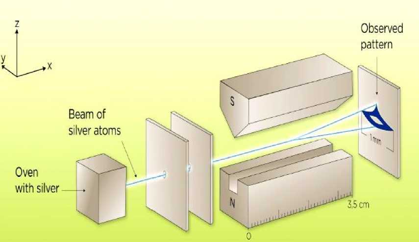
Fig. 1. A schematic picture of the Stern-Gerlach experimental set up
We choose the z axis. Suppose that the result of the first N trials is N + ( + )'s and N_ ( - )'s .
Q : What can we say now?
Example . Given a density matrix p , parameterized as above, the rules of quantum mechanics tell us that the probability that a measurement of the spin along the z axis will yield ( + 1) is
P (^z =+1|p) = Tr 1 (1 + ^z ) p = 1 (1 + z)
where a. is a Pauli matrix, and the probability that this measurement will yield ( - 1) is
P (^z =-1| P ) = Tr 1 (1 - ^z ) P = 1 (1 - z ) .
Now we use Bayes’ theorem. The hypothesis is H = ”the quantum state is within a volume d p centered on p ”. We have assigned this hypothesis a prior probability P ( H ) = p ( p ) d p . The data D is a string of N + ( + )' s and N_ ( - )' s , in a particular order; each of the N = N + + N_ outcomes is assumed to be independent of all the others. Using the definition of independence, we see that the likelihood is
1 1 N + Г 1
2 ( 1 + z ) ] [ 2 ( 1 - z )
F(DH) = [P(az = +1|p)]N* [P(az =-l|p)]"
Applied Bayes’ theorem, we get the posterior probability
F ( HD ) = F ( D )- 1 2 ( 1 + z )
N +
N
-(1 - z) p(p)d p,
where P ( D ) = J 1 (1 + z )
N +
1 1 N
— ( 1 - z ) p ( p ) d p . When the number of trials N is large, and the
prior probability p ( p ) is a slowly varying function, the posterior probability F ( H |D ) has a sharp peak at
N- N z = z =-------. Thus, after a large number of trials in which e measure a , we can be confident of the exp z value of the parameter z in the density matrix of the system.
Remark . The only people who will not be convinced of this are those whose choice of prior probability p ( p ) is strongly biased against the value z = zex . Furthermore, those who do not agree can be identified a priori by noting that their prior probabilities are strong functions of p . In choosing p ( p ) d p , we can use the principle of indifference, applied to the unitary symmetry of Hilbert space, to reduce the problem to one of choosing a probability for the eigenvalues of p . There is, however, no compelling rationale for any particular choice; in particular, we must decide how biased we towards pure states.
Remark . We have argued that, in a Bayesian framework, the nature of our ignorance about a quantum system can often be more faithfully represented by a prior probability p ( p ) d p over the range of allowed density matrices, rather than by a specific choice of density matrix. This method is particularly appropriate when (i) the preparation procedure may favor a direction in Hilbert space, but we do not know what that direction is, and (ii) we can recreate the preparation procedure repeatedly, and perform measurements of our choice on each prepared system. In this case, as data comes in, we use Bayes’ theorem to update p ( p ) d p . Eventually, all but strongly biased observers (who can be identified a priori by an examination of their choice of prior probability) will be convinced of the values of the quantum probabilities. In this way, initially subjective probability assignments become more and more objective. Caves et al in [1] regarded p ( p ) d p as a measure rather than a probability. This approach required them to prove, first, a quantum version of the Finetti theorem [2], and, second, that Bayes’ theorem can be applied to p ( p ) d p , Both steps become unnecessary if we treat p ( p ) d p as, fundamentally, a probability.
Example . We can orient the Stern-Gerlach apparatus along different axes (see, Fig. 1). If we choose the x axis or the y axis, the relevant predictions of quantum mechanics are
|
P (ax = +1| p ) = Tr 1 ( 1 + a x ) p = 1 ( 1 + x ) |
P ( a x = - 1| p ) = Tr 1 ( 1 — a x ) p = 1 ( 1 — x ) |
|
P ( a y = + 1l p ) = Tr 1 ( 1 + a y ) p = 1 ( 1 + У ) |
P ( a y = -1l p ) = Tr 1 ( 1 - a y ) p = 1 ( 1 - у ) |
For each trial, we can choose whether to measure ax,a,, or a _. Then, if the outcomes include N x y z + z measurements of a. with the result az = +1, and so on, the posterior probability becomes
P (HD )=P (D )-1 П j = x, У,z

N - j p ( A ) d p ,
where P ( D ) is given by obvious integral. Clearly when the number of trials is large, we have determined the entire density matrix to the satisfaction of all but strongly biased observers. Our subjective of probabilities have led us to an objective conclusion about quantum probabilities.
Q : If we assign an impure density matrix p to a quantum system, does this not already take into account our ignorance about it?
Q: Why is it preferable to assign, instead, a probability p ( p ) d p to the set of possible density matrices?
The answers on these questions depend on the nature of our ignorance. Let us consider an example.
Example: Probabilities for density matrices vs. density matrices. Suppose the system is the spin of an electron plucked from the air. Then we expected that the state p = ^ I will describe it, in the sense that if we do repeated trials (plucking a new electron each time, and measuring its spin along an axis of our choice), we will find that xexp
N + - — N —
N + ■ + N —
„ N + y — N — y .
- , y ex „ ^ —------ -, and z.
exp
- - + y — y
N + z - N — z
'exp N. + N ’
+ z — z
and all tend to zero.
Suppose instead that the spin is prepared by a technician who (with the aid of a Stern-Gerlach device) puts it in either a pure state with a = + 1 , or a pure state with ax = + 1 , and each time decides which choice to make by flipping a coin that we believe is fair. In this case the appropriate density matrix is
1 (1+a) +12V z J 2
1 (1 + a)
2 x
1 ( 3 1л
4 1 1 1V
Comparing with p =
( 1 + z
v - + iy
- — iy
1 — z >
, we see that we now expect
x exp, y exp, and z exp to approach
+ —, 0, and + — , respectively. Now suppose that the spin is prepared by a technician who puts it in either a pure state with a = +1, or a pure state with ax = +1, and makes the same choice every time. We, however, are not aware of what her choice is. If forced to assign a particular density matrix, we would have to choose as above mentioned.
However, the situation is clearly different from what it was in the previous example. In the present case, repeated experiments would not verify as above mentioned density matrix p , but would instead converge on either vn = 0 and z^n = +1, or xn = +1 and zpvn = 0 . Therefore, in this case, it is more appropriate to exp exp exp exp assign a prior probability of one-half to
p =
1 ( 1 + a )
and a prior probability of one-half to
p =
1 ( 1 + a )
. Then, as data comes in, we can update these probability assignments with Bayes’ theo-
rem, as described above.
Thus, it is better to choose p ( p ) d p when it is possible that there is something about the preparation procedure that consistently prefers a particular direction in Hilbert space, but we do not know what direction is. Since this possibility can rarely out a priori , we are typically better served by choosing a priory probability p ( p ) d p , rather than a particular value of p itself.
Suppose we have decided to choose a prior probability p ( p ) d p for the density matrix p of some quantum system.
Q : How should we choose this probability?
Example : Non-informative priors for density matrices . In the case where we have little or no information about the quantum system, we would like to formulate the appropriate analog of the principle of difference . Consider a qunit, a quantum system whose Hilbert space has dimension n that is known to us. We can always write the density matrix (whatever it is) in the form p = U p U , where U is unitary with determinant one, and p is diagonal with nonnegative entries px ,..., pn that sum to one. There is a natural measure for special unitary matrices, the Haar’s measure; it is invariant under U ^ CU , where C is a constant special unitary matrix.
In the simplest case of n = 2 , we can parameterize U as following:
U = exp {iaa} exp {ia2^ } exp {iaa }, with 0 < a < n, 0 < a < “ n, 0 < a - n ; then the normalized
Haar’s measure is
dU = n ”2 sin ( a ) d a d a d a . This construction is extended to all n . Suppose we know that the state of the quantum system is pure. Then we can set p. = Sn Sj x, and parameterize p via U . Then it is natural to choose d p = dU and p ( p ) = 1 , because this is the only choice that invariant under unitary rotations in Hilbert space.
Now consider the more general case where we do not have information about the purity of the system’s quantum state.
Example . We define the volume element via d p = dUdF , where dU is the normalized Haar’s measure for U , and dF = ( n — 1 ) S ( px +...+ pn — 1 ) dpx.. pn is normalized measure for the pt ’s that we will call the Feynman measure (because the same integral appears in the evaluation of one-loop Feynman diagrams). In last equation assumes that each pt runs from zero to one; then p = U pU is an overcomplete construction, because U can rearrange the p ’s. This is easily fixed by imposing px >...> pn , and multiplying dF by n ! . However, equation for dF as it stands is easier to write and think about; the overcompleteness of this construction of p causes no harm. In the case n = 2 , we previously chose
3 n 1
d p = dV = — dxdydz for the parameterization. In this case, the eigenvalues of p are — ( 1 + r ) and
( 1 — r ) , with 0 < r < 1 . After integrating over U , dV ^ 3 r 2 dr ; in comparison, dF = dr for this case. The purity of a density matrix p can be parameterized by Trp 2, which for n = 2 is ^-( 1 + r 2 ) . Thus the volume measure dV is more biased towards pure states than is the Feynman measure dF ; we have dV = 3 ( 2Tr p 2 — 1 ) dF . In general, we can accommodate any such bias taking p ( p ) d p to be of the form: p ( p ) d p = p ( Trp2 ) dUdF , where p ( x ) is an increasing function if we are biased towards having a pure state. Unfortunately, there does not seem to be a compelling argument towards any particular choice of the function p ( x ) , including p ( x ) = 1 . Once we have done enough experiments, our original biases become largely irrelevant, as we saw above.
The state is often characterized by the set of moments {^}, i.e., numbers generated by the state according to the following rule: ^ = nnk^ = ^nkpn . Combining the first and the second moments, we n obtain the variance An2 = ^n2^ — ni^2. Its root, An , called the standard deviation or the uncertainty, characterizes deviations from the mean value, i.e., fluctuations.
Example . For instance, for a regular die, ( n ) = 3.5 and A n = 1.7 , while for state ( 3.1.1 ) , nip = 5.85 and A n = 0.73 . Having the full set of moments, one can, in principle, reconstruct the state, i.e., the probabilities. (This is not always true in quantum models that see below).
Any possible state of the die can be depicted as a point in the 6D space of states. The frame of reference for this space should be given by the axes pn or cn = pp . In the last case, the depicting point belongs, due to the normalization condition, to the multi-dimensional sphere 5 , and the state vector can be written as p = { c } (for comparison with the Poincare sphere S2 , see below).
Now let N = 2 . One can imagine a coin made of magnetized iron. Due the magnetic field on the Earth, the probabilities of the heads, p+ , or tails, p = 1 — p +, depend on the value and direction of magnetization. Each individual coin can be characterized by a state у = ( p+ , p ) .
Measurement of a classical state
For a state у , which is prepared by means of a certain procedure and therefore known, one can predict the outcomes of individual trials. However, these predictions only relate to probabilities, with the exception fro the case where one of the components of у equals 1. One can pose the inverse problem of measuring the state у .
Clearly, it is impossible to measure у for a given coin in a single trial. (Speaking of a trial, we mean a “fair“ throw of the coin with the initial toss being sufficiently chaotic). For instance, “tails” can correspond to any initial state except у = ( p+ = 0, p = 1 ) , where the index of у denotes the number of trials M . One should either throw one and the same coin many times or make a large number of identically prepared coins, a uniform ensemble . If the coins remain the same, are not damaged in the course of trials, then all these ways to measure the state are equivalent (the probability model is ergodic ).
Example . From the viewpoint of measurement, the only way to define the probability is to connect it with the rate of corresponding outcome. Throwing a coin 10 times and discovering “heads” each time, one can state, with a certain extent to confidence, that у « у 0 = ( 1,0 ) . However, it is possible that the next 90 trials the coin will show “tails“. This time, we will be more or less confident that у « у 00 = ( 0.1,0.9 ) , -and still we can be mistaken, since the actual state might be, say, у = ( 0.5,0.5 ) .
This example of exclusive bad luck shows that an actual (prepared) state у cannot be measured with full reliability. One can only hope that as M increase, the probability of a large mistake falls and ум approaches the actual value у . In other words, relative rates of different outcomes almost always manifest regularity for increasing M .
Hence, for the case of known preparation procedure, the state у (the set of probabilities) can be associated with the chosen individual object. Here the state is understood as the information about the object allowing the prediction of the probabilities of different events. At the same time, for the case of known measurement results, the state can be only associated with an ensemble of similarly prepared objects, always with some finite reliability. There is no principal difference between a single trial and number of trials: the results of experiments are always probabilistic. Similar conclusions can be made in the quantum case.
Example: Analogue of a mixed state and the marginals. Consider two sets of coins prepared in the states у'= (p‘,p‘) and у = (p‘,p"). The numbers of coins in the sets are denotes by N' and N" (N’ + N'' = N). If the coins are randomly chosen from both sets and then thrown, the “heads“ and “tails“ will evidently occur with weighted probabilities p'N' + p N"
N
p’N' + p"N" N
which are determined by both the properties of the coins and the relative numbers of coins in the sets, and . In this case, double stochasticity appears: (i) due o the random choice of the coins; and (ii) due NN to the random occurring of “heads“ and “tails“.
This is the simplest classical analogue of a mixed state in quantum theory (in its first definition, see below). Clearly, such a mixed state cannot be associated with an individual system; it is a property of the ensemble containing two sorts of coins. In quantum theory, this corresponds to a classical ensemble of similar systems being in various states with some probabilities.
Remark . In quantum theory, there also exists another definition of a mixed state. This definition characterizes a part of the degrees of freedom for a quantum object; in the classical theory, it corresponds to marginal probability distributions, or marginals. Marginal distributions are obtained by summing elementary probabilities, in accordance with Kolmogorov’s additivity theorem. Hence, they can be considered as a property of an individual object. For instance, for a die, one can determine the marginal probabilities of odd and even numbers, pp , and p . For the state ( 3.1.1 ) , we obtain p+ = 0.97 , and p = 0.03 .
Example : Moments and probabilities . Now let two coins from different sets be thrown simultaneously. We introduce two random variables 5 ,, S^ taking values S j , s2 = ± 1 for “heads” or tails“, respectively. The system is described by a set of probabilities p ( s t, s 2 = ± 1 ) of four different combinations ( ± 1, ± 1 ) . If the coins do not interact and are thrown independently, then the “2D” probabilities p ( s t, s 2 ) are determined by the products of the corresponding 1D probabilities p ( s t, s 2 ) = p ( s t) p ( s 2 ) . However, let the peculiarities of the throw or the interaction between the magnetic moments of the coins lead to some correlation between the results of the trials. Then the state of the two coins is determined by the set of four elementary probabilities p ( S j , s 2 ) . The marginal probabilities and the moments are obtained by summing,
pk ( sk ) = p ( sk,+1) + p ( sk,-1),
(Sk) = p (+1)-p (-1) = 2 p (+1)-1 (k = 1,2) .
к SS2) = Г (+1,+1) + p (-1,-1)- p (+1,-1)- p (-1,+1)
Hence, ISSk )| < 1,1(SS )| < 1. In the simple case considered here, one can easily solve the inverse problem, which is called the problem of moments. In other words, one can easily express the probabilities in terms of moments, pk (sk ) =1 (1 + SM.)),
p ( s 1 , s 2 ) ^p^ ( 1 + S 1 ( S 1) + s 2 ( S 2) + S 1 s 2 ( S 1 S 2 )) .
From above condition and the condition p ( s t, s 2 ) > 0 , it follows that the moments are not independent; they must satisfy certain inequalities. Provided that the first moments S are given, the correlator (SS 2 ) cannot be arbitrary large or small, f ^ < ( SS ) < f ^.
Here fmin = max (-1 - (S1) - (S2), - 1 + (S1) + (S2 )) , fmax = min (1 + (S1) - (S2M - (S1 ) + (S2 )) .
For instance, for ^Sj) = ^S2 ) , we have the limitation 2|^Sj| — 1 < |(SS2 )| < 1. In particular, the corre- lator cannot equal zero
for K s J J > ^ (i.e., for p + > 0.75 ).
In the quantum theory, analogous inequalities for quantum moments F , which are obtained by averaging with respect to the wave function (WF), F^ = ^ | F | ^ ), are sometimes violated. Paradoxes of these kind cases will be discussed below. Note that in such cases, the notion of elementary probabilities has no sense, and the quantum probability model can be called non-Kolmogorovian .
Quantum probabilities
The classical models described above have little connection with quantum physics. The “state” of a die can include not only the properties of this die, as we supposed above, but also the parameters of the initial toss. (According to classical dynamics, these parameters unambiguously determine the outcome).
Remark . Stochasticity appears here as a result of variations in the value and direction of the initial force. (Under certain additional conditions, such models manifest dynamical chaos ). Quantum stochasticity is believed to have a fundamental nature; it is not caused by some unknown hidden variables, though Einstein could never admit that: “God plays dice“. It is an astonishing feature of quantum probability models that in some cases, there exist marginals but there are no elementary probabilities. This feature can be called the non-Kolmogorovianess of the quantum theory; in the general case it corresponds to the absence of a priori values of the observables (see in details below). For instance, one can measure (or calculate using wave function (WF) ψ ) coordinate and momentum distribution for a particle at some time moment, but their joint distribution cannot be measured. Reconstruction of the joint distribution from the marginals is ambiguous and sometimes leads to negative probabilities. Therefore, it is natural to assume that a particle has no a priori coordinates and momenta.
Remark . It is also important that classical models have no concept of complex probability amplitudes and hence, do not describe quantum interference and complex vector spaces of states. There is no classical analogue of non-commuting variables, which do not admit joint probability distributions.
Four basic topics can be considered in this case: ( i ) the logical structure of quantum description; ( ii ) the necessity of distinguishing between a theory and its interpretation; ( iii ) the WF: its sense, preparation, modulation, measurement, and reduction; and ( iv ) “non-locality“ of quantum physics, i.e., the impossibility of introducing joint probabilities for non-commuting operators. In this connection, non-classical experiments must be discussed.
Remark . The physical meaning of the basic quantum mechanical concepts (such as the WF, reduction, state preparation and measurement, the projection postulate, and the uncertainty principle) can be clarified using realistic experimental procedures and employing classical analogies whenever possible. In all known experiments, excellent agreement is observed between the prediction of the quantum theory and the corresponding experimental data. Unfortunately, the efficiency of the quantum formalism is accompanied by difficulties in its interpretation, which have not yet been overcome. In particular, there is still no common viewpoint on the sense of WF. Another important notion of quantum mechanics, the WF reduction, is also uncertain. Two basic types of understanding can be distinguished among a variety of viewpoints. A group of physicists following Bohr consider the WF to be a property of each isolated quantum system such as, for instance, as ingle electron (the orthodox, or Copengagen, interpretation). The other group, following Einstein, assumes that the WF describes an ensemble of similar systems (the statistical, or ensemble, interpretation). Nine different interpretations of the quantum formalism are considered in [1]. Among many other studies devoted to methodological problems of quantum physics, it is also worth mentioning in [1 – 7].
The sense of some basic notions in non-relativistic quantum physics can be clarified using the operational approach, i.e., demonstrating how these notions manifest themselves in experiments.
Here we mostly focus on dynamical experiments connected with evolution of quantum systems in space and time. As a typical example, we consider the Stern-Gerlach experiment where particles with magnetic moment M are deflected in an inhomogeneous magnetic field.
Example. In 1922, Stern and Gerlach performed an experiment, passing electrons through a strong, inhomogeneous magnetic field. Figure 1shows the structure of the Stern-Gerlach physical experiment. In this case, S is the source of particles, F is a screen with a pinhole (collimator), F is a domain with an inhomogeneous magnetic field, D is a photographic plate. The elements F and F perform spatial and magnetic filtering and can be considered as parts of the preparation and measurement sections of the setup, respectively. If D contains a pinhole, then F and D work as a filter, which sometimes transmits particles in the state with definite spin projection. Using this example, one can clearly specify the basic elements of a dynamical experiment: the source of particle S, the detectors D (crystal of silver bromide contained in the photosensitive film), the space between S and D where quantum evolution of the particle takes place, and the filters F , F . The source S and the collimator F (a screen with a pinhole for spatial selection) form the preparation part of the setup. The magnet F provides the inhomogeneous magnetic field that couples the spin and kinetic degrees of a particle. Together with the detectors D, the magnet can be considered as the measurement part of the setup. In such a scheme, only the evolution of a particle between the source and the detector is described by the Schrodinger equation accounting for the classical magnetic field. S, F , F and D are supposed to be classical devices with known parameters.
Thus in the classical probabilistic model, events (e.g., word occurrences, category memberships, relevance, location, task, genre) are represented as sets and the probability measure is based on a set measure, e.g., set cardinality. In contrast, in quantum probability, events are represented as orthonormal vectors and the probability measure is the trace of the product between a density matrix and the matrix representing an event as summarized in Table 1.
Table 1. The correspondence between classical probability and quantum probability
|
Notion |
Classical |
Quantum |
|
Event space Random event Probability Measure |
Q Set Set measure |
Hilbert vector space "Ы Orthonormal basis {|S), |H)} State vector |y>) |
The simple example in Fig. 2 depicts that when vectors are used to implement both events and densities the probability in the vector space is the squared inner product between the vectors, that is, the squared size of the projection of A onto ϕ .
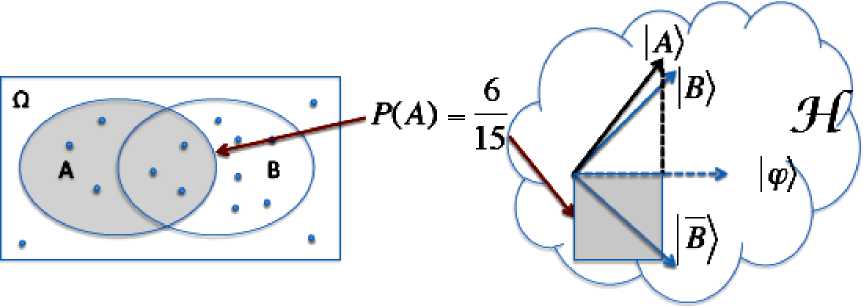
Fig. 2. The correspondence between classical probability and quantum probability
An important recurring theme is the unusual, non-classical properties of quantum mechanics.
But what exactly is the difference between quantum mechanics and the classical world?
Understanding this difference is vital in learning how to perform information processing tasks that are difficult or impossible with classical physics [3 – 6].
Appendix conclude a brief discussion of the Bell inequality, a compelling example of an essential difference between quantum and classical physics.
Appendix 1: EPR paradox, Bell inequality and Kochen-Specker theorem
A1.1.Einstein –Podolsky – Rosen (EPR) - Paradox and Non-locality in Quantum Mechanics
When we speak of an object, we assume that the physical properties of that object have an existence independent of observation. That is, measurements merely act to reveal such physical properties. As quantum mechanics was being developed in the 1920’s and 1930’s a strange point of view arose that differs markedly from the classical view.
-
(1) According to quantum mechanics, an observed particle does not possess physical properties that exist independent of observation.
-
(2) Rather, such physical properties arise as a consequence of measurements performed upon the system.
Remark A1.1 . For example, according to quantum mechanics a qubit does not possess definite properties of “ spin in the z direction , σ ”, and “ spin in the x direction , σ ”, each of which can be revealed by performing the appropriate measurement. Rather, quantum mechanics gives a set of rules, which specify, given the state vector, the probabilities for the possible measurement outcomes when the observable σ , is measured, or when the observable σ is measured.
Albert Einstein [with Nathan Rosen and Boris Podolsky (EPR)] proposed a thought experiment which, he believed, demonstrate that quantum mechanics is not a complete theory of Nature.
The essence of the EPR argument is as follows. EPR were interested in what they termed “elements of reality”. Their belief was that any such element of reality must be expressed in any complete physical theory. The goal of the argument was to show that quantum mechanics is not complete physical theory, by identifying elements of reality that were not included in quantum mechanics. The way they attempt to do this was by introducing what they claimed was a sufficient condition for a physical property to be an element of reality, that it be possible to predict with certainty the value that property will have, immediately before measurement.
Example A1.1 . Consider, for example, an entangled pair of qubits belonging to Observable 1 and Observable 2 , respectively: ψ = ( 01 - 10 ) . Suppose Observables 1 and 2 are a long way away from 2
one another. Observable 1 performs a measurement of spin along the ϑ axis, that is, he measures the observable 9 • d" . Then a simple quantum mechanical calculation (see, below ) shows that he can predict with certainty that Observable 2 will measure (– 1) on his qubit if he also measures the ϑ axis. Similarly, if Observable 1 measured (– 1), then he can predict with certainty that Observable 2 will measure (+1) on his qubit. Because it is always possible for Observable 1 to predict the value of the measurement result recorded when Observable 2’s qubit is measured in the ϑ direction, that physical property must correspond to an element of reality, by the EPR criterion , and should be represented in any complete physical theory.
However, standard quantum mechanics, as we have presented it, merely tells one how to calculate the probabilities of the respective measurement outcomes if 9 • c r is measured. Standard quantum mechanics certainly does not include any fundamental element intended to represent the value of 9 • c , for all unit vectors ϑ .
Remark A1.2 . The goal of EPR was to show that quantum mechanics is incomplete , by demonstrating that quantum mechanics lacked some essential “element of reality”, by their criterion. They hoped to force a return to a more classical view of the world, one in which systems could be ascribed properties which existed independently of measurements performed on those systems. Unfortunately ( for EPR ), most physicists did not accept the above reasoning as convincing. The attempt to impose on Nature by fiat properties, which she must obey seems a most peculiar way of studying her laws. Nearly thirty years after the EPR paper was published, an experimental test was proposed that could be used to check whether or not the picture of the world which EPR were hoping to force a return to is valid or not. It turns out that Nature experimentally invalidates that point of view, while agreeing with quantum mechanics. The key to this experiment invalidation is a result known as Bell’s inequality.
Bell’s inequality is not a result about quantum mechanics, so as recommended in [2] “the first thing we need to do is momentarily forget all our knowledge of quantum mechanics”.
Remark A1.3 . To obtain Bell’s inequality, we’re going to do a thought experiment, which we will analyze using our common sense notions of how the world works – the sort of notions EPR thought Nature ought to obey. After we have done the common sense analysis, we will perform a quantum mechanical analysis, which we can show is not consistent with the common sense analysis. Nature can then be asked, by means of a real experiment, to decide between our common sense notion of how the world works, and quantum mechanics.
Example A1.2 : Experiment description . We perform the following experiment, illustrated in Fig. A1.1.
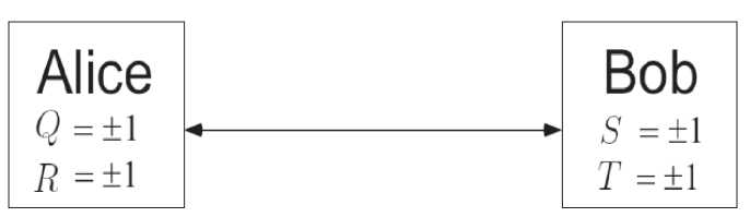
Fig. A1.1. Schematic experimental setup for the Bell’s inequalities
Observable 1 receives one particle and performs a measurement on it. Imagine that Observable 1 has available two different measurement apparatuses, so he could choose to do one of two different measurements. Observable 1 can choose to measure either Q or R , and Observable 2 chooses to measure either Q or R . They perform their measurements simultaneously. Observables 1 and 2 assumed to be far enough apart that performing a measurement on one system can not have any effect on the result of measurements on the other. These measurements are of physical properties which we shall label P and P , respectively. Observable 1 doesn’t know in advance which measurement he will choose to perform. Rather, when he receives the particle he flips a coin or uses some other random method to decide which measurement to perform. We suppose for simplicity that the measurements can each have one of two outcomes, (+1) or (1). Suppose Observer’s 1 particle has a value Q for the property P . Q assumed to be an objective property of Observer’s 1 particle, which is merely revealed by the measurement. Similarly , let R denote the value revealed by a measurement of the property P .
Similarly, suppose that Observer 2 is capable of measuring one of two properties, P or P , once again revealing an objectively existing value S or T for the property, each taking value, (+1) or (- 1). Observer 2 does not decide beforehand which property he will measure, but waits until he has received the particle and then chooses randomly. The timing of the experiment is arranged so that Observers 1 and 2 do their measurements at the same time (or, to use the more precise language of relativity, in a causally disconnected manner). Therefore, the measurement which Observer 1 performs cannot disturb the result of Observer’s 2 measurement (or vice versa ), since physical influences cannot propagate faster than light. We are going to do some simple algebra with the quantity QS + RS + RT — QT .
Example A1.3: Bell inequalities. Notice that
QS + RS + RT — QT = (Q + R)S + (R — Q )T. (A1.1)
Because R, Q = ± 1 it follows that either ( Q + R ) S = 0 or ( R — Q ) T = 0 . In either case, it is easy to see that QR + RS + RT — QT = ± 2 . Suppose next that p ( q , r , 5 , t ) is the probability that, before the measurements are performed, the system is in a state where Q = q , R = r , S = 5 , and T = t . These probabilities may depend on how Observer 3 performs his preparation, and on experimental noise. Letting M ( ■ ) denote the mean value of a quantity, we have
|
M ( QS + RS + RT — QT ) |
= |
У p ( q, r , s , t )( qs + rs + rt — qt ) q , r , s , t |
|
< |
У p ( q , r , s , t ) x 2 q , r , s , t |
|
|
= |
2 |
(A1.2)
Also,
|
M ( QS + RS + RT - QT ) : = : У p ( q , r, s , t ) qs + У p ( q , r, s, t ) rs : : q , r , s , t q , r , s , t |
|
|
i + i У p ( q , r , s , t ) rt - У p ( q , r , s , t ) qt : : q , r , s , t q , r , s , t |
. (A1.3) |
|
: = : M ( QS ) + M ( RS ) + M ( RT ) - M ( QT ) |
Comparing (A1.2) and (A1.3) we obtain the Bell inequality ,
M ( QS ) + M ( RS ) + M ( RT ) - M ( QT ) < 2 . (A1.4)
This result is also often known as the CHSH inequality .
It is a part of a larger set of inequalities known generically as Bell inequalities.
By repeating the experiment many times, Observers 1 and 2 can determine each quantity on the left hand side of the Bell inequality. For example, after finishing a set of experiments, Observers 1 and 2 get together to analyze their data. They look at all the experiments where Observer 1 measured P and Observer 2 measured P . By multiplying the results of their experiments together, they get a sample of values for QS . By averaging over this sample, they can estimate M ( QS ) to an accuracy only limited by the number of experiments, which they perform. Similarly, they can estimate all the other quantities on the left hand side of the Bell inequality, and thus check to see whether it is obeyed in a real experiment.
Example A1.4 : Analysis of Bell inequalities . It’s time to put some quantum mechanics back in the picture. Imagine we perform the following quantum mechanical experiment. Observer 3 prepares a quantum system of two qubits in the state
| 0 = 1= ( 01) - 110) ) . (A1.5)
He pass the first qubit to Observer 1 , and the second qubit to Observer 2 . They perform measurements of the following observables:
|
Q = z 1 |
S = ^ ( - Z 2 - X 2 ) |
|
R = Xi |
T = ^ ( Z1 - X 2 ) |
Simple calculations show that the average values for these Observables , written in the quantum mechanical notation (•), are:
|
(QS^ = ^2 |
(RS ) = V2 |
(RT ) = X 21 |
(QT ) = 2i |
Thus,
(QS ) + ( RS ) + ( RT ) - ( QT ) = 272 . (A1.6)
From Eq. (A1.4) we see that the average value of QS plus the average value of RS plus the average value of RT minus the average value of QT can never exceed two. Yet here, quantum mechanics predicts that this sum of averages yields 222 .
Example A1.5: Tsirelson’s inequality. Boris Tsirelson raised the question whether quantum theory imposed an upper limit to correlations between distant events (a limit which would of course be higher than the classical one, given by Bell’s inequality). Suppose Q = q ■ ст, R = 7 • 57, S = 7 • 57, T = t • <5, where <7, r, s and t are real unit vectors in three dimensions. In this case
(Q ® S + R ® S + R ® T — Q 0 T )2 = 41 + [Q, R ]0[S, T ] (A1.7)
For any two bounded operators A and B , we have general inequalities as
II[A B]hl|AB|| + 1 BAI < 2|A||||B||, and therefore, in the present case, I [Q, R ]s 2,1 [S, T ]s 2.
It thus follows from Eq. (A1. 7) that || 4 1 + [ Q , R ] ® [ S, T ] || < 8 or
(Q^ + ( RS ) + ( RT ) - QH^ < 272 . (A1.8)
This is Tsirelson’s inequality. Its right hand side is exactly equal to upper limit that can be attained by the left hand side of CHSH inequality (A1.7). So the violation of the Bell inequality found in Eq. (A1.6) is the maximum possible in quantum mechanics. Quantum theory does not allow any stronger violation of the CHSH inequality than the one already achieved in Aspect’s experiment.
Clever experiments using photons – particles of light – have been done to check the prediction (A1.6) of quantum mechanics versus the Bell inequality (A1.4) which we where led to by our common sense reasoning. The results of experiments were resoundingly in favor of the quantum mechanical prediction. The Bell inequality (A1.4) is not obeyed by Nature.
A1.2. The Logical Backgrounds of Quantum Non-Locality and Hidden-Variable Theory: Einstein – Podolsky – Rosen Paradox and Bell’s Inequalities
Consider some “elementary” events A, B, C , . , such as “ the electron spin in the x — direction is up ”, as well as some of the joints of these propositions; e.g., AB, AC,. „ , ABC,. „ . In order to be consistently interpretable, the probability of these events P ( A ), P ( B ), P ( C ), . , P ( AB ), P ( AC ), . , P ( ABC ),... must satisfy some inequalities of the probability theory; for example:
P(A) + P(B) — P(AB) < 1 or P(A) — P(AB) — P(AC) + P(BC) > 0. (A1.9)
These inequalities are satisfied for every possible classical probability distribution P These inequalities are investigated in the middle of the 19 th century George Boole and referred to them as conditions of possible experience .
Remark A1.4 .The number and complexity of the inequalities increase fast as the number of events grows. Among them are the famous inequalities that arise in the Einstein-Podolsky-Rosen (EPR)-experiment and its generalizations. In particular, Bell inequalities and Clauser-Horne (CH) inequalities (see, Section A1.1 ).
Consider, for example, the Bell inequalities and its physical meaning. The logical and mathematical formalism is described below.
A1.2.1. Local realism, EPR-experiment and Bell inequalities (Simplified cases)
Local realism is a world view which holds that physical systems have local objective properties, independent of observation. It implies constraints on the statistics of two widely separated systems. These constraints, known as of Bell inequalities, can be violated by quantum mechanics. The Clauser – Horne – Shi-mony – Holt (CHSH) Bell inequalities applies to a pair of two-state systems and constraints the value of a linear combination of four correlation functions between the two systems. Quantum mechanics violates the CHSH inequality; the violation has been confirmed experimentally.
The essence of Bell inequalities is related to Einstein’s notion of “realism”: that an object has “objective properties” whether they are measured or not. Bell inequalities, in their simplest form, reflect constraints on the statistics of any three local properties of a collection of objects. Consider a set of objects, each characterized by three two-valued (or dichotomic) properties a , b , and c . Then, grouping the objects as a function
n(.,.) of two (out of the three) properties (for instance grouping together objects having property a but no b ), it is easy to build a simple inequality relating the number of objects in various groups defined by different pairs of properties. For example,
n (a, —।b) < n (a, — c )+n (—b. c).
(A1.10)
While such an inequality only refers to the simultaneous specification of any pair of properties, its satisfaction depends on the existence of a probability distribution for all three . Thus, even when the three properties cannot be accessed at the same time (for whatever reason), Eq. (1) still holds provided that there exists such an objective description of each object using three parameters a , b , and c ; therefore, Eq. (A1.10) provides a straightforward test of “local realism ” (i.e., the combination of objectivity and locality). As confirmed experimentally [8], an equality such as Eq. (A1.10) can be violated in quantum mechanics. It is the uncertainty principle (implying that the simultaneous perfect knowledge of two conjugate observables is impossible), which is at the root of such a violation. Argument similar to those above are used to derive the Bell inequalities and the Clauser-Horne-Shimony (CHCH) inequalities, and their violation can be traced back to the nonexistence of an underlying joint probability distribution for incompatible variables [4].
Example A1.6: Bell states. For all single qubit states | a ) and | b ) we have | ^ ^ | a)| b . We say that a state of a composite system having this property (that it can’t be written as a product of states of its component system) is called an entangled state .
Let’s us consider slightly more complicated circuit, shown in Figure A1.2, which has a Hadamard gate followed by a CNOT operation, and transforms the four computational basis states according to the table
—j= ( 0} + 11) ) 0} , and then the
given. As an explicit example, the Hadamard gate takes the input 00 to
CNOT gives the output state
—j= ( 00} +11^). Note how this works: first, the Hadamard transform puts the top qubit in a superposition; this then acts as a control input to the CNOT, and the target gets inverted only when the control is 1. The output states
Table A1.1: Bell states
|
1 A ») = 4 (00) + ln>) |
1 a = ^ ( 00) -111)) |
|
1 A.) = ^ ( 01) +1 10) ) |
1 A.)=^ ( 01) -1 10) ) |
(A1.11)
are known as the Bell states, or sometimes the EPR states or EPR pairs, after the people – Bell, and Einstein, Podolsky, and Rosen – who first pointed the strange properties of states like these. The mnemonic notation | во \ | A oi^ | во \ | A i) may be understood via the equations
I = ^ ( °- У + (- 1 ) x l 1, — y! ) , where — y is the negation of y , x , y e { 0-1 } .
(A1.12)
In 00
Out
( 00) + 111 )
( 01 + 110) )
( 00)-111 )
( 01 -110) )
о
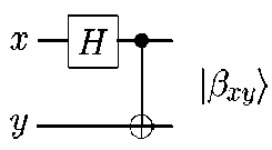
Fig. A1.2: Quantum circuit to create Bell states, and its input – output quantum “truth table”
Example A1.7: Anti – correlation in the EPR experiment . Suppose we prepare the two state
| ^ = —/=( 01) — 110^ ) , a state sometimes known as the spin-singlet for historical reasons. This
state is an
entangled state of the two qubit system. Suppose we perform a measurement of spin along the
*
^—
9 axis on
both qubits, that is, we measure the observable 9- — = 9— + 9— + 9— on each qubit, getting a result
of+1 or -1 for each qubit. It turns out that no matter what choice of 9 we make, the result of the two measurements are always opposite to one another. That is, if the measurement on the first qubit yields +1, then the measurement on the second qubit will yield (–1), and vice versa. It is as though the second qubit knows the result of the measurement on the first, no matter how the first qubit is measured. To see why this is true, suppose | a ) and | b ) are the eigenstates of 9 - <— — . Then there exist complex numbers a , в , y , 5 such that । o^ = a a + в b and i = y a + 5 b •
Substituting we obtain
I Vх) = ^=( 01) — 110) ) = -y=(a5 — Py)( ab — bbo))
e
i e
But ( a5 — в5 ) is the determinant of the unitary matrix
a
У
в 5
, and thus is equal to a phase factor
for some real e . Thus
|
1 ^ = T? ( |
01—110 ) - ( |
ab ) — |
ba ) |
, up to an unobservable global
phase factor. As a result, if a measurement of 9 - —— is performed on both qubits, then we can see that a result of +1 (- 1) on the first qubit implies a result of -1 (+1) on the second qubit, i.e., we are observed the anti – correlation in the EPR experiment.
Example A1.8: Bell inequalities derivation. Consider two widely separated entangled systems in general, more specifically, a pair of spin — — particles in singlet state (so-called Bohm’s version of EPR pair, see, Table A1.1): |вц) = |^ = —t=(01) — 110)). Assume that an observer, acting independently on each
particle, can measure the spin component of that particle along two possible orientations, for example with Stern-Gerlach setup. Let the first observer either measure the z component of one of the particle (and call this observable A and the outcome of the measurement a ) or else the component along an axis making an angle e with the z axis (observable B , with outcome b). Correspondingly, the second observer measures (on the second particle) either the z component (observable A') or else the component making an angle ф with the z axis (observable C ). Locality implies that the two distant observers have no influence on each other, i.e., the decision to make one of the two possible measurements on the first particle does not effect the outcome of the measurement on the other particle. Indeed, it is known that the marginal statistics of the outcome of the spin measurement on the second particle, c for instance, is unchanged whether one measures A or B on the first particle. Let us now outline a general derivation of conventional Bell inequalities [1, 2]. Consider three dichotomic random variables A , B and C that represents properties of the system and can only take on the values (+1) or (-1) with equal probability ^—^ . For our purpose, they stand of course for the measured spin components (either up or down along the chosen axis), i.e., the Bell variables. (As A' is fully anticorrelated with A (see, Example A1.7), we do not make use of it.) any random set of outcomes a ,b , and c must obey
ab + ac - bc < 1
(A1.13)
along with the two corresponding equations obtained by cyclic permutation ( a ^ b ^ c ) . Indeed, the lefthand side of Eq.(3) is equal to +1 when a ] = b ], while it is equal to |- 1 ± 2| when [ a = — b . Taking the average of Eq. (A1.13) and its permutations yields the three Bell inequalities:
|
aab^ + ( ac ) - ( bc) |
< 1 |
|
aab} - aac} + ( bc) |
< 1 |
|
- ( ab ) + ( ac ) + ( bc) |
< 1 |
(A1.14)
relating the correlation coefficients between pairs of variables.
Two last equations in (A1.14) can be combined in the form of standard Bell inequalities: |(ab ) - acc^ | + bcc^ < 1 .
Remark A1.5 . The important point is that inequalities (A1.14) involves only the simultaneous specification of two (out of the three) random variables, although it is assumed that the three variables possess an element of reality, i.e., they can in principle be known at the same time (even if not on practice). In other words, it is assumed that there exists an underlying joint probability distribution P ( a , b, c ) , in which case the Bell inequalities (which depend only on the marginal probability P ( a, b ) = ^ P ( a , b , c ) and cycle
c permutation) must be satisfied. Therefore, the violation of any of the inequalities (A1.14) implies that a ,b , and c cannot derive from a joint distribution (i.e., cannot be described by any local hidden-variable theory). In the following, we will show that the violation of Bell inequalities, while ruling out such a classical underlying description of local realism, still does not contradict a quantum one based on an underlying joint density matrix pABc, but forces the corresponding entropies to be negative.
Remark A1.6 . It is known that quantum mechanics cannot be reduced to any non-contextual hidden-variable theories. This means that the probability space of outcomes of measurements changes according to what is measured. A hidden-variable theory with such many probability spaces is often called a contextual hidden-variable theory. In such a theory, we usually consider that the change of the probability space is due to the interaction between the object and the measuring apparatus. Bell argues that in the EPR-Bohm Gedankenexperiment , this interpretation leads us to an unacceptable conclusion. He insists that if the Bell inequality is not satisfied, then there exists action - at - a distance in the EPR-Bohm Gedankenexperiment. Several EPR-Bohm type experiments have already been performed since then and violations of Bell type inequalities have been observed. As a result, it has been widely believed that quantum mechanics has a non – local character such as action - at - a distance . It is hardly known, however, that several authors showed that the violation of the Bell inequalities did not always mean existence of the “ action - at - a distance” , making local models that violate the Bell inequalities.
Remark A1.7 . The Bell inequalities are written in terms of correlations between two-state systems. The CHSH inequality tested in the most recent experiments [involves four quantities, two from each two-state system, it constrains the value of a linear combination of the four measurable correlation functions of these 22
quantities, and it follows from the assumption of a joint probability for the four quantities. Its violation by two spin- particles in a spin-singlet state reflects the tight correlation between the spins. The CHSH inequality is thus closely analogous to the information Bell inequality (see, below Eq. (A1.15)). For the orientations considered above, however, the CHSH inequality is violated over a large range of angles than is equality (A1,15). Thus the Bell inequality (A1.15) does not reveal all quantum behavior that is inconsistent with local realism. This realization prompts us to consider what is that Bell inequalities test. A Bell inequality – whether for correlations or for information – is a consequence of our assuming a joint probability for a set of measurable quantities. When quantum mechanics violates a Bell inequality, it means, strictly speaking, only that the quantum statistics cannot be derived from such a joint probability. A Bell inequality is transformed into a test of local realism by the argument that objectivity and realism ensure the existence and relevance of the joint probability. Violation is thus interpreted as a conflict either with objectivity or with locality.
Remark A1.8 . If Bell inequalities arise from a joint probability, why not take a more direct approach? Start with marginal probabilities predicted by quantum mechanics, and ask if they can be derived high-order joint probabilities. This approach has been advocated by Garg and Mermin , who formulate it mathematically and investigate it for pairs of spin- s systems for several values of s . The Garg-Mermin approach ferrets out all the consequences of local realism for arbitrary systems, but it is not simple mathematically, nor does it yield clear-cut constraints for experimental test . The CHSH inequality is simple to derive and has been tested, but it does not test all the consequences of local realism, nor is it easy to generalize nontrivially to other than two-state systems. Thus we see a role for information Bell inequalities: They do not get at all the consequences of local realism, but they are simple to derive and applicable to arbitrary systems; as such, they can be a useful tool for the comparison of quantum mechanics against the requirements of local realism
Conclusions
What does mean ? It means that one or more of the assumptions that went into the derivation of the Bell inequality must be incorrect. Vast tomes have been written analyzing the various forms in which this type of argument can be made, and analyzing the subtly different assumptions, which must be made to reach Bell – like inequalities. Here we merely summarize the main points.
There are two assumptions made in the proof of (A1.4) which are questionable:
Po , PR , P. , Pa Q.R.S.T
-
(1) The assumption that the physical properties Q R S T have definite values ^, , , , which exist independent of observation. This is sometimes known as the assumption of realism.
-
(2) The assumption that Observer 1 performing his measurement does not influence the result of the Observer’s 2 measurement. This is sometimes known as the assumption of locality.
These two assumptions together are known as the assumptions of local realism . They are certainly intuitively plausible assumptions about how the world works, and they fit our everyday experience. Yet the Bell inequalities show that at least one of these assumptions is not correct.
What we can learn from Bell’s inequality ? The most important lesson is that we deeply held commonsense intuitions about how the world works are wrong. The world is not locally realistic . Bell’s inequality together with substantial experimental evidence now points to the conclusion that either or both of locality and realism must be dropped from our view of the world if we are develop a food intuitive understanding of quantum mechanics.
What lessons can the fields of quantum computation and quantum information learn from Bell’s inequality ? By throwing some entanglement into a problem we open up a new world of possibilities unimaginable with classical information. The bigger picture is that Bell’s inequality teaches us that entanglement is a fundamentally new resource in the world that goes essentially beyond classical resources; ”iron to the classical world’s bronze age.” A major task of quantum computation and quantum information is to exploit this new resource to do information processing tasks impossible or much difficult with classical resources.
References Intelligent it for student education in quantum informatics. Pt 1: logic of classical / quantum probabilities
- Хренников А.Ю. Квантовая физика и неколмогоровские теории вероятностей. - М.: КнигоРус, 2008.
- Nielsen M.A., Chuang I. L. Quantum computation and quantum information. - Cambridge Univ. Press, 2010.
- Schmitt I. Quantum query processing: unifying database querying and information retrieval. - Otto-von-Guericke-Universitat Magdeburg, 2006.
- Pitowski I. Quantum probability and quantum logic. - Springer, Heidelberg, 1989.
- Jaeger G. Developments in Quantum Probability and the Copenhagen Approach // Entropy, 2018. - Vol. 20. - № 420. - Pp. 1-19.
- Ellerman D. Logical Entropy: Quantum logical information theory // Entropy, 2018. - Vol. 20. - № 679. - Pp. 1-22.
- Stuart T.E., Slater J.A., Colbeck R., Renner R., Tittel W. Experimental bound on the maximum predictive power of physical theories // Physical Review Letters. - 2012. - Vol. 109. - № 2. - Pp. 020402.
- Norsen T. On the explanation of Born-Rule statistics in the de Broglie-Bohm pilot-wave theory // Entropy, 2018. -Vol. 20. - № 422. - Pp. 1-26.
- Wennerstrom H., Westlund Per-Olof. A quantum description of the Stern-Gerlach experiment // Entropy, 2018. -Vol.19. - No186. - Pp 1-13.
