Intelligent Rate Adaptation Based on Improved Simulated Annealing Algorithm

Published Online November 2010 in MECS

Through the modulation and coding, IEEE802.11 a /b/g in the PHY layer can provide a variety of variable rates, such as the IEEE802.11b protocol provides four types of rates which are 1Mb/s, 2Mb/s, 5.5Mb/s and 11Mb/s, but in the MAC layer, the current protocol only fix the rate for the specified frame type, and do not fix the switching approach between the four rates. Therefore, it can not effectively use the adaptive switching between the rates, which makes it impossible to provide maximum use of the PHY layer rate. As the development of wireless communications, smart antennas, digital signal processing technology, etc. the physical layer can provide a very high rate, such as the 802.11n standard can reach 100Mbps speed for users. However, in [1] [2] the throughput of 802.11 DCF MAC protocol has the theoretical limit, for high-speed wireless LAN, it is not enough to only increase transmitting rate in Physical layer, but also needed to reduce the overhead of MAC layer protocol and do research on rate adaptation in MAC layer protocol.

At present, there are two types of rates adaptive methods. An algorithm is ARF (Auto Rate Fallback) [3] [4]. It is the method commonly used commercially. The other is RBAR (Receiver Based Auto Rate) algorithm [5]

Manuscript received January 1, 2011; revised January 1, 2011; accepted January 1, 2011.

Corresponding author:     Lianfen Huang; E-mail:

• [6] . Compared with the ARF, RBAR algorithm can respond channel’s change faster, but when there is no hidden terminal or exposed terminal, it will increase the overhead of the system.

The proposed SAARF (Simulated Annealing Auto Rate Fallback) algorithm in this paper is compatible with the ARF. The main idea is the simulated annealing from artificial intelligence. Through a certain probability and statistics, it makes node faster recover rate after the congestion in the network, thereby improving network performance.

• II.    The Basic Principles Of Saarf Protocol

• A.    The Basic Principle of ARF Protocol

ARF is based on the statistical success of the number of received ACK frames to determine the channel’s condition. In the ARF protocol, if the sender does not receive two consecutive ACK frames, the channel quality is assumed to be deteriorated, so the sender chooses a lower transmitting rate and starts a timer; if the sender consecutively and successfully received 10 ACK frames, or the timer expires, the channel is assumed to be improved, which will increase the transmitting rate to the next high level. The limitations of the method is not well reflecting the changes of channel quality in real time, on the other hand, ARF always view 10 as the threshold to determine the increase of the rate, which will affect its performance. Such as some nodes transmitting with a high rate for a long term decrease rate because of sudden congestion, they still need to receive 10 consecutive ACK to increase rates, if these high-speed node increase rate when the ACK frame number is less than 10, it is possible to improve the network performance in some extent.

• B.    The Basic Principle of Simulated Annealing Algorithm

Simulated annealing algorithm is an optimization strategy from artificial intelligence in the computer science field. Its most important feature is to receive a new solution according to Metropolis criterion [10] [11] [12]. Metropolis criterion not only receives optimal solution, but also receives deterioration solution with probability. The probability of receiving deterioration solution is decreasing with the decrease of the temperature T0. When T0 is close to 0, the probability of receiving deterioration solution is also close to 0, so the algorithm can only receive the optimal solution. It is considered that the algorithm starts with a solution, through continuous cooling, finally obtaining the optimal solution, which is also the process of the slow convergence. In addition, the length of Mapkob chain in the simulated annealing algorithm produced the number of new solutions under temperature T0, the more numbers of new solutions, the larger scope of solutions searched, but on the other hand the more time consumed for the algorithm, which causes delay of the node for sending a packet and affects network performance.

The SA algorithm could be described by the following pseudo-code:

• 1.    choose an initial solution X0 randomly

• 2.    give an initial temperature T0, X= X0, T=T0

• 3.    while the stop criterion is not yet satisfied do

• 4.    for i=1 to L do

• 5.    pick a new solution X ' randomly

• 6.        A f = f ( X ') - f ( X )

• 7.    if A f < 0 then X = X '

• 8.    else X = X 'with probability exp(- A f / T0)

• 9.    T0 = g(T0)

• 10.    return X

In this pseudo-code, X represents solution, f ( X ) represents the target function, and L is Mapkob chain. Function g ( ) is a decreasing function, it controls T0 to be smaller and smaller till it closed to 0, and its general type likes T0 = T0 * factor, the common value of this factor is 0.95~0.90. Obviously, the algorithm would return a better solution in an acceptable time eventually.

• C.    The Basic Principle of the SAARF Protocol

The basic idea of SAARF is expressed by the following state diagram:

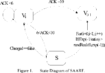
In Fig. 1, the vi and vi+1 respectively represent the low-rate state and the next high-rate state. S represents the intermediate state in SAARF, it changes to state vi or vi+1 according to whether the condition is established or not. L is the length of the Mapkob chain; it controls the numbers of the comparison in the loop. The variable changed represents whether increasing rate has occurred by the comparison, its initial value is false, if the node has increased rate, the value of changed is true, otherwise, the value of changed is false.

When a node is in state v , if the number of ACK frame is less than 6, the state transition would not happen, if the ACK frame number satisfies the inequality 6

- 1/- v +L

When in state S, comparing e ^{v num} and rand

Real(0, e ) in the loop body whose loop count is L, If

• - 1/- v ±L

e 'num > rand Re al(0, e-1) , then the node transits to the next high-rate state vi+1 ; if the number of comparisons reaches to L, and the rate is still not being promoted, that is variable changed is false, then back to the state vi .

In the v_i state, if the node received 10 consecutive ACK frames, SAARF is the same as ARF, as the rate will be increased by one grade,

And the function expression corresponding to the state diagram is:

V 1

v i + 1

ACK = 10

V H v i + 1

，

— 1/ ' "1

6 <  ACK <  10, e v num >  rand Re al (0, e ^-1)

v i        ， else

This can be seen, SAARF is the protocol that added S state on the basis of ARF, it makes the node has a faster transition to the higher rate.

III. The Performance Analysis Of Saarf Protocol

SAARF algorithm is an improvement of ARF, it can be divided into two parts: one part is the original ARF algorithm, which is the part of receiving the optimal solution; the other part is about simulated annealing algorithm, based on probability of receiving deterioration solution parts. This paper set Vnew as the new solution, Vold as the old solution, the three features of the SAARF are:

• •    When the received ACK number is 10, it is viewed as Vnew > Vold, so increase the rate to the next high rate.

• •    When 6  randReal(0,exp(-1)), it increases the rate. Otherwise, it keeps the current rate unchanged for transmitting. Ratio is the proportion that the transmitting number of the next higher rate takes up in the total transmitting number of all the rates.

• •    The total number of the node’s transmitting rate is Vnum; the Vnum is equivalent to the temperature T0 in simulated annealing, as the number of sending packets increases, the Vnum continuously increases. Thereby, the node could know the optimal solution through the slow convergence.

• A.    The Rate Analysis of SAARF:

  -1/ v i +L

Let the probability of e v™ >  rand ^Re al (0, e ) be pe, , then:

e - 1/ ratio

^P e ⁼ e

e ratio

Let the length of Mapkob chain be L, while in the chain, the probability of is

If a node’s four types of transmitting rate are nearly 25%, and the length of Mapkob chain is 1, we get:

P, = 0.018316 p_M = 0.018316 p„ = 0.142048 e                         Me                         te

Similarly, we know the probability of using SAARF for rapid increase is only 14%. Therefore, if a node ’ s four types of transmitting rate are nearly 25%, SAARF algorithm and the original ARF is not very different, overall network performance is relatively close.

• B.    The Throughput Analysis of SAARF

Let the time of sending data be T_DATA , the time of sending ACK be T_ACK , the time wasted to transmit PLCP

Header and Preamble be T_PLCP , the time of DIFS be T_difs (50us), the time of SIFS be T_sifs and the time of delay in transmission be delay .

PMe = Pe + (1 - Pe )Pe + (1 - Pe )2 Pe ++ (1 - Pe )"-’ Pe = £0 - Pe )i Pe i=0

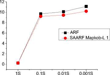
In the condition 6

of transmitting a frame is

time T_DATA

Supposing the node’s ACK numbers satisfies the inequality 6V_i to V_{i+ 1} through SAARF is:

T

DATA

= T r PLCP

+ (28 + ^) x 8

V

Pte = (PMe^{+ (1 -}PMe ) PMe^{+ (1 -}PMe )2 PMe ) = E ⁽¹- PMe У PMe i=⁰                .(3)

Where N is the number of bytes to be sent in data packets, 28 is the result of the length of MAC Header (24Bytes) plus 4Bytes of the CRC check. The throughput is:

The expectation value of the node’s rate is:

v = V₊1 ■ Pe⁺V^(1-Pe).          (4)

It equals to:

v = ^Vi ^{+ (}vi+1 ^{- V}i)Pte

In the ARF protocol, under the condition of 6v_i , so its expectation rate is:

^v = Vi

From (5) and (6) can be seen:

Because (v_i+1- vi)Pe is always greater than 0, the expectation value of node’s transmitting rate using SAARF protocol is larger than that of using ARF.

If a node’s rate is 2Mb/s at this time, and the received ACK number is greater than 6 and less than 10, the next transmitting rate of 5.5Mb/s in the proportion of the total number of all the transmitting rate is 40%, that is ratio=40%, according to the above:

P_e = 0.223130 p_m = 0.223130 p„ = 0.531138 e Me te

From p_te , it is informed that the probability of the node’s rapid increasing for rate is 53%, which is relied on SAARF. It is indicated that the node is probable to have a rate of 5.5Mb/s to send the next data packet. Thereby, when the number of a transmission rate in the proportion of the total number is 40% to 50% or more, rapid promotion through the SAARF appears very likely.

C =

N x 8

TdifS^{+ CW +}TDATA^{+ dela}y⁺Tsif⁺TACK^{+ delay}

If V SAARF > V ARF then T_D^S_A^A_T^A_A^RF< T_D^A_A^R_T^F_A， we can see the through put of SAARF is larger than that of ARF.

The essence of SAARF is to achieve the rapid increase of node’s rate through probability and statistics. Using SAARF protocol, it is suitable for most nodes to increase rate. It reflects the tendency of the node’s rate change. However, the channel is changeable, a few nodes do not adapt to the changes in the channel in real time after lifting rate, which is equivalent to receive the deterioration solution in simulated annealing. Node would decrease rate after not receiving two consecutive ACK frames, which affects the transmission rate and throughput of the node. Although individual nodes will be affected, overall, the network throughput and average transmission rate is rising.

• C.    The Pseudo-Code Analysis of SAARF Protocol

In QualNet, the file named mac_dot11-sta.h should be modified to make the SAARF protocol. The function MacDot11StationAdjustDataRateForNewOutgoingPacke tis is the primary-function concerning about controlling the rate adaptation in wireless network. The SAARF protocol could be described by the following pseudo-code:

• 1.    switch (node’s dataRateType)

• 2.    {

• 3.    make statistics about every kind of rate numbers and the total rate numbers

• 4.    }

• 5.    use ARF approach to control rate adaptation

• 6.    the added part by SAARF is from now on:

• 7.    if( node numAcksInSuccess satisfy the condition greater than 6 and less than 9)

• 8.    switch (node’s next high rate type)

• 9.    {

• 10.    case (node’s next rate)

• 11.{

• 12.    for ( i to L(Mapkob Chain Length))

  -1/ -^±1

• 13.    if ( e ^vnum > randReal(0,e¹) )

• 14.{

• 15.           rate promotes to the next high level rate

• 16.           break;

• 17.}

• 18.break

• 19.}

• 20.    }

• 21.    if ( node’s rate has been promoted)

• 22.    { set node firstTxAtNewRate = TRUE

• 23.    numAcksFailed = 0

• 24.    numAcksInSuccess = 0

• 25.    reset dataRateTimer

• 26.    }

From the pseudo-code above and the Mapkob chain, it is easy to know that the time complexity of the algorithm is O(n), which means that the algorithm could be solved in polynomial time. So it would not cost much time to implement SAARF. Meanwhile, the space complexity of SAARF takes up very few memory of the node, even less than 1KB memory. Compared to the current nodes (whatever computer or mobile phone etc.), it could all easily satisfy the condition of running the SAARF protocol.

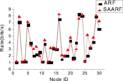
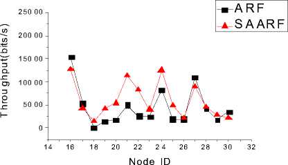
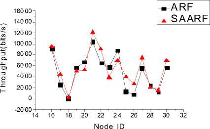
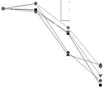
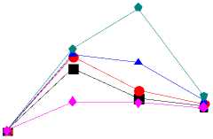
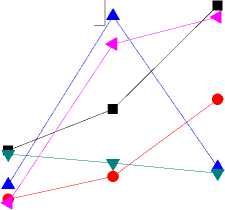
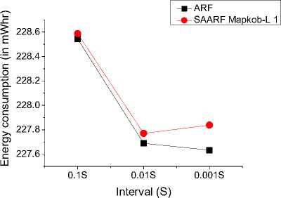
IV.    The Simulation And Analysis Of Saarf

• A.    The Scenario’s Setting of the Simulation

In QualNet3.9.5 simulation environment, randomly

TABLE I.

THE PARAMETERS OF SIMULATION SCENARIO

Items to Send 100 Item Size (bytes) 521 Interval 1S Start Time 1S End Time 25S Enable Rsvp-Te? No generating 30 nodes, making 15 CBR flows according to the order of 1-30, 2-29, 3-28… 15-16

The parameter Interval in the simulation changes in the range of 1S, 0.1S, 0.01S, 0.001S, the shorter the interval is, the sender will send more packets in unit time, the more likely to receive sufficient number of ACK before the timer timeout. Once the number of ACK is larger than 6 and less than 10, there may be rapid increase of rate. On the other hand, if the sending interval is too short, there will be a large number of packets in the network in unit time, which may cause network congestion dramatically, resulting in a large number of ACK timeout. When there are two ACK timeout, the sender will decrease the rate, starting the next round of rate adaptation.

• B.    The Analysis of the Rate Comparison between SAARF and ARF

We chose the interval for 0.1S, the length of Mapkob chain is 1, comparing the average rate of transmitting data for each node. It is shown below:

Fig. 2 shows, after using SAARF, the average transmitting rate for most of nodes is higher than the average transmitting rate of nodes using ARF. but there

Figure 2. Interval is 0.1S, the average rate of each node for transmitting data are also a few nodes, the average rate is slightly lower than the average rate of ARF, which is likely to the situation of receiving deterioration solution in simulated annealing, some nodes rapidly raise the rate through the Metropolis criterion, after lifting the rate, they immediately decrease the rate because of two consecutive ACK not received, which results the decreasing of the average transmitting rate for packets.

• C.    The Analysis of the Throughput Comparison between SAARF and ARF

in the case of the length of the Mapkob chain is 1, the time interval were selected for the 0.01S and 0.001S, each simulation runs ten times, and take the mean value. The throughput of each receiving node is shown below:

Figure 3. Interval is 0.01s, the throughput of each receiving node

Figure 4. Interval is 0.001s, the throughput of each receiving node

random number, make the nodes which should not raise rates occasionally promote its rate, lead to the occurrence of packet loss and network congestion, and affect the entire network throughput. In addition, if Mapkob length is too long, the time wasted on algorithm execution becomes longer, which would delay the time of sending packets, resulting the decline of the throughput.

• D.    The Analysis of the Jitter Comparison between SAARF and ARF

0.70.60.40.30.1

Jitter is a kind of significant element in network performance measurement. It could reflect the stability of a network. From QualNet 3.9.5, with the Mapkob chain value L ∈(1,5,10,20), it could compare jitter of the ARF and SAARF, the figure is shown below:

Fig. 3 and Fig. 4 show, the throughput trend of SAARF and ARF is similar, but in certain peak point, SAARF has a higher value, this is because SAARF could make high-speed node increasingly easy to return to high-speed transmission. But there are some nodes, whose throughput is slightly lower than the throughput of ARF, this is because of receiving deterioration solution, after the raise of the rate, the rate and channel conditions are not favorable, so decreasing the rate again, which results the decline of the throughput. Despite a few nodes’ throughput decrease, the overall throughput of the network is rising.

Now change the length of Mapkob chain in SAARF, let the value L ∈(1,5,10,20), and compare the throughput of the four cases under SAARF with the original ARF.

< 0.2

1S

0.1S

Iterval (s)

0.01S    0.001S

Figure 6. Jitter of SAARF and ARF

—■— ARF

• — •— SAARF Mapkob-L 1

• —    А — SAARF Mapkob-L 5

• —    ▼— SAARF Mapkob-L 10

• - ♦— SAARF Mapkob-L 20

15000 14000 13000 12000

5 11000 10000 9000

О) 8000 о 7000 6000

I- 5000

4000 3000

1S

0.1S      0.01S    0.001S interval

• ■ ARF

• • SAARF Mapkob-L 1

• -А-SAARF Mapkob-L 5

• • SAARF Mapkob-L 10

♦ SAARF Mapkob-L 20

Figure 5. Throughput of SAARF and ARF

Fig. 5 shows, if Mapkob length are 1, 5 and 10, the average throughput of SAARF are better than that of ARF protocol. When Mapkob length is 10, the system throughput obtains the best value, when Mapkob length is 20, he throughput of the system is the smallest. Overall, with the length of Mapkob chain increases, the throughput of the system increases, but when Mapkob length is too long (in the Fig. 5, the length is 20), the throughput declines. This is because Mapkob chain controls the number of times for comparing with random number. When the number is proper, it will quickly make the transition from v_i to v_i+1 , and does not affect network performance. But when the number is too large, it may increase the probability of the e^{-1/ ratio} larger than

Fig. 6 shows, generally, the larger the Mapkob chain is, the higher jitter the network performs. So, the jitter of network which runs SAARF with the value of L being 20 is always higher than that of the network whose L value is smaller than 20. Meanwhile, when the interval is 0.1S or 0.01S, the jitter performed by SAARF is not always smaller than that by ARF, but sometimes it is bigger than that by ARF. Such as SAARF with Mapkob-L 5, when the interval is 0.01S, the jitter is smaller than ARF, but when interval is 0.1S, and Mapkob-L is 1, its average jitter is a little bigger than that of ARF. It seems that there is no rule to determine whose jitter should be smaller or bigger than that of ARF; every kind of SAARF with different Mapkob chains owns its best jitter value in the situation of different intervals. But when the interval is 0.001S, the four kinds of average jitter are larger than that of ARF. Combining the situation of the throughput and jitter of SAARF and ARF, it is obvious that SAARF could still positively affect the performance of network.

• E.    The Analysis of the ACK Numbers in SAARF

ACK number is an important parameter in rate adaptation, only the ACK number reaches the pre-set threshold, could the rate adaptation system run. In ARF protocol, the ACK number is set to be 10, once the number reaches 10, In this paper, the lower limit of ACK number to run SAARF is set to be 6, while, the lower limit could also be set to be smaller than 6, such as 3, 4,5, etc. or larger than 6, such as 7,8,etc. In this experiment, the Mapkob chain is set to be 10, under this situation, the comparison of the throughput is shown:

Thus, when L∈(1,5,10,20) and the interval∈(0.1S, 0.01S, 0.001S), the comparison performs like:

■ SAARF Mapkob-L 10

2 6000

i-

ACK number

Figure 7. Throughput of SAARF When Variable is ACK Number

4L

J?

0) Q

0) О) го

Ф

<

11.2

11.0

10.8

10.6

10.4

10.2

10.0

9.8

9.6

9.4

9.2

9.0

■ ARF

-♦- SAARF Mapkob-L 1

-^- SAARF Mapkob-L 5

-▼-SAARF Mapkob-L 10

-N SAARF Mapkob-L 20

0.1S

0.01S

0.001S

Interval (S)

Through Fig. 7, under the situation of Mapkob chain is 10, it is clear that when ACK number is 5, the throughput is the largest, with the ACK number increasing, the throughput is decreasing. In this paper, we choose 6 as the lower limit of ACK number. It is just a kind of value, other value could also be set for it, but every kind of situation must have a best value matching the largest throughput. Though it is hard to find, generally, the common value would always be greater than or equal to 5 and be less than or equal to 7. Because if it is too small, the rate increasing would happen too early, it could bring negative effects on network. But if it is too large, the advantage of SAARF could not perform in time. So, a moderate value is a better choice to implement the SAARF algorithm.

• F.    The Analysis of Delay in ARF and SAARF

Delay measurement is also a major element in network performance, the comparison between the delay of ARF and the delay of SAARF when Mapkob chain is 1 is below:

Interval (S)

Figure 8.   Delay of ARF and SAARF

From Fig. 8, it is clear that when the interval turns from 1S to 0.001S, no matter ARF or SAARF, the Delay would also increase. However, the delay of SAARF is a little lower than ARF, which means that when Mapkob chain is 1, SAARF performs better than ARF in delay measurement.

Figure 9.   Delay of ARF and SAARF

Fig. 9 shows, when interval is 0.1S or 0.001S, the delay performance of SAARF are always better than that of ARF, whatever L is 1,5,10 or 20. But when the interval is 0.01S, the SAARF does not always perform better than ARF, it also performs worse. When L is 20, the explanation of worse situation maybe that L value is too big and the algorithm costs too much time, which causes the severe delay; but when L is 5, the delay could not have a strong reason why it is worse than ARF, and some research would still be needed to carry on.

• G.    The Analysis of Energy Consumption in ARF and SAARF

There is no doubt that energy consumption is a very important element that should be considered seriously, especially in our modern society, almost every government or organization appeal people to save energy and use energy reasonably. The SAARF protocol should also consider energy consumption, under the scenario described above; the sum of the total energy consumption of 30 nodes with the situation of interval belonging to (0.1S, 0.01S, and 0.001S) is below:

Figure 10. Energy Consumption of ARF and SAARF

From Fig. 10, it is seen that the energy consumed by SAARF is larger than that by ARF. Besides, with the interval becoming smaller, the gap between SAARF and

ARF becomes larger. Additionally, it is worth noticing that the unit is mWhr. When the size of the nodes is not so large, the energy consumption of SAARF would not bring more negative effects, but when the size of nodes is very large, the energy consumption problem would affect our decision whether to use SAARF or not; after all, it consumes more energy.

On the other hand, although SAARF may consume more energy, it also raises throughput, and partially reduces the jitter and delay. So, building a network is a kind of thing which needs overall consideration, individual element can affect building a network, but can not absolutely affect that.

V.    Conclusion

The SAARF protocol described in this article is based on the ARF protocol and is improvement to ARF. The SAARF applies the simulated annealing algorithm in artificial intelligence to rate adaptation in MAC layer for the purpose of achieving rapid rate promotion. Using the SA algorithm, it makes the rate adaptation process more intelligent and it seems like every node is wise enough to know when to quickly promote its rate. With the simulation results, it is confirmed that the simulated annealing algorithm is useable in MAC layer’s rate adaptation, and SAARF could be applied in 802.11 WLAN (Wireless Local Area Network). Similarly, other algorithms in artificial intelligence field could also be applied in rate adaptation in wireless network, such as GA (Genetic Algorithm), ACO (Ant Colony Optimization) algorithm, PSO (Particle Swarm Optimization) algorithm etc. they all could be modified and improved to adapt to the specific environment in wireless network, it could be expected that these algorithms would be used widely to solve similar problems, and artificial intelligence would also be largely introduced to wireless network. After all, it provides an intelligently approach to handle the complicate objects, thus making things more easily controlled than before. Besides, it used a kind of method from computer science field to resolve the problem in communication field, it is a good try, and we will continuously make related research on the field of wireless network.