Intergovernmental Allocation of Public Resources, Fiscal Decentralization and Economic Growth

Published Online June 2011 in MECS

The relationship between government expenditures and economic growth has been long in research. Reference [1] initially found a significant positive relationship between total government expenditures and the output. Reference [2] examed the impacts of government expenditures on consumption and capital accumulation to the output separately and found that government expenditures on consumption has a smaller while still positive impact on the output. On the basis of this paper, Reference [3] incorporated government expenditures into the standard endogenous growth model which was traced to [4]. The empirical study in [3] provided ambiguous conclusions on the impacts of different parts of government expenditures on the output. Reference [5] distinguished between productive and non-productive government expenditures, by using a panal data of 43 developing countries they found a short-term positive while a longterm negative impact of productive expenditures on the output. Reference [6] paid attention to the impact s of different government structures on the economy, while the empirical study of them was criticized by [7] about the time span of the panal data they used.

The above papers provided valuable insights into the relationship between government expenditures and economic growth. Different intergorvernmental allocation of public resources is needed to discuss, when talking about government expenditures or fiscal decentralization and economic growth. Meanwhile, distinguishing between productive and non-productive government expenditures is needed as their impact are different in a short term. Gvernment structures should be considered if there are differences among the contributions of each level government expenditures to the output. In this paper we established an endogenous growth model extended from [8] and incorporated a two-level government structure into it as the basic model in Section II. In Section III, intergovernmental transfer payments are assumed to extend the basic model. Section IV extended the basic model with another intergovernmental allocation of public resources, i.e. revenue autonomy of the local-level government. Section V concluded this paper.

• II.    The Basic Model

• A.    Government Structures

In a closed economy with only governments and identical economic agents, government expenditures are supposed to maximize the consumer welfare. Here in the basic model, government structures are important because productivety may be different related with each level government expenditures. Two levels, governments of the state-level and the local-level, are supposed for simplicity. Government expenditures are divided consequently into those from the state-level government and from the local-level governments, f denoted the former and S the latter. The whole government expenditures hence, denoted by g, satisfies g = f + S                    (1)

We assume that government expenditures are all financed contemporaneously by a flat-rate income tax, and a balanced budget constraint holds for the whole government implies g = T = т • y                   (2)

where T is the tax rate in (2). Expression (2) means that the government can neither finance deficits by issuing debt nor run surpluses by accumulating assets, that is so called a balanced budget. Governments assign their revenue in the way that a proportion of ф e [0,1] is decentralized to the local-level governments, then government expenditures can be identified as f = (1 - фТ               (3a)

5 = фт у                  (3b)

• B.    The Production Function

The production function of the economy is the function of capital and government expenditures, and assumed to be a CES production function as f (k, f, 5) = f (k, g) = (ak- Z + в- Z + Y-Z)-1/Z (4) where y is output per worker, k is capital per worker, α, β and γ are the output elasticity of k, f and s respectively, α + β + γ=1 guarantees a constant returns to scale of the economy. Meanwhile, the elasticity of substitution 1/(1 + Z) is constant and let Z ^ -1 for simplicity in (4).

• C.    The Utility Function

The representative, infinite-lived household in a closed economy seeks to maximize his lifetime utility, as given by

*

U = J_o u ( c ) e - "dt

where c is consumption per person, u(c) is an continuous, differentiable instantaneous utility fuction of identical consumers and 0 <  p < 1 is the discount rate in (5).

Population, which corresponds to the number of workers and consumers, is constant. For simplicity and without loss of generality, the instantaneous utility function takes the form as

1- C 1

u ( c ) = c-^¹              (6)

1 - C

Given (1)~(6), a simple caculation yields the capital growth constrains as k = (1 - t)y - c                 (7)

The problem of an identical consumer is to maximize (5) subject to (7).

• D.    The Balanced Growth Path

On the balanced growth path, all variable grows at the same rate, called the steady-state growth rate. In order to compute the steady-state growth rate, we construct a Hamilton function as

H = c ' + Л[(1 - t)y - c]

1 - C

The two conditions are given by c" = X(9a)

X = pX - Xa (1 - t )( a k - ^Z + e f - ^Z + У ? - ^Z ) + ^Z )/ ^Z k~^Z 1 (9b)

Integrating (9a) and (9b), we have the consumption growth rate on the balanced growth path as c = a (1 - t ) R (X) - p(10)

where R(X) = {a + [в(1 - ф)-Z + Уф-Z ](g / k)-Z }-(1+Z)/Z is satisfied in (10). The same growth rates of capital and the output provide a constant government expenditure-capital ratio on the banlanced growth path,g/k, as g / k = {a /[tz - в(1 - ф)-Z - УФ"Z ]}-1/Z      (11)

Integrating both (10) and (11) yields

a (1 - t ) T - в (1 - Ф ) ^{- Z} - уф ' 1 (^{1 + Z} )/ ^Z p (12)

G =—-- ■■ ----- ^- °

Expression (12) represents that the steady-state growth rate ( G ) is the function of all parameters and variables. The maximization problem of consumers equals to maximize the steady-state growth rate represented by (12).

• E.    Fiscal Decentralization and Economic Growth

In the basic model, the portion that is decentralized to the local-level governments ( ф ) reflects both the revenue and expenditure portion of the local-level governments. We could use this variable as the indicator of fiscal decentralization. Under the assumptions of the basic model, we have Proposition 1 to represent the relationship between fiscal decentralization and economic growth.

Proposition 1. In a closed economy with two-level governments and the Cobb-Doglas production function , holding all other parameters constant,

• a)    The optimal degree of fiscal decentralization equals to the ratio between the contribution of local public expenditures on the output ( у ) and the contribution of all public expenditures on the output ⁽в + у).

• b)    There is an “Inverted U-shape” relationship between fiscal decentralization and economic growth. .

Proof.

• a) In order to show how fiscal decentralization affect economic growth, we could differentiate both parts of (12) with respect to ф yields

  5 G / 5 ф =

  
  

a (1 - t )(1 + Z )( «t^z ) + ^Z )/ ^Z УтФ ^-х*^Z ) - в (1 - Ф > + ^Z ) ] (13) a [ t^z - в (1 - ф ) ^{- Z} - Уф ^Z I ^Z

Given that Z >-1 and assuming that G > 0 in (13), the nonnegative right hand side of (13) requires уф”(1+Z) - в(1 - ф)-(1+Z) > 0

A simple caculation yields л f A 1/(1+Z)

ф <(Y]

1 - ф l в J

The optimal fiscal decentralization rate is the one as

\ 1/(1 + Z )

ф =1у I

• 1 - ф  l в J

A simple expression of (16) considering the Cobb-Doglas production function. Let z =-1, expression (16) implies ф'= в + У

b) A simple caculation of (13) gives that when ф <  ф ,

5G / дф > 0 implies that the steady-state growth rate increases as the degree of fiscal decentralization increases. While when φ> φ∗ , ∂G/ ∂φ< 0 implies that the steadystate growth rate decreases as the degree of fiscal decentralization decreases. There is an “Inverted U-shape” relationship between these two variables on the balanced growth path.

That completes the proof of Proposition 1.

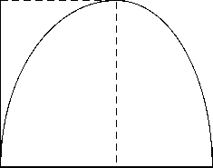
Fig. 1 shows the “Inverted U-shape” relationship between fiscal decentralization and economic growth.

G

G

φ ^∗ =   ^{β l}

β l + β c

φ

Figure.1. The “Inverted U-shape” relationship between fiscal decentralization and economic growth

As the degree of fiscal decentralization increases from zero to one, the long-run growth rate increases at first and arrived at the maximum value, then it decreases eventually. The implication is obvious. A lower degree of fiscal decentralization constrains the power of the locallevel government, while a greater degree of fiscal decentralization increases the externality costs of public goods provided by each local-level government. The optimal degree of fiscal decentralization are denoted by (17).

• III.    Extension of The Basic Model: Intergovernmental Transfer Payment

• A.    Intergovernmental Transfer Payments

Public resources gathered should be allocated among all level governments. Different allocation will have different impact to the economic growth.

First and the most popular form of intergovernmental allocation of public resources is intergovernmental transfer payments. A transfer payment, denoted by T , is given by the higher-level government to the lower-level government in many coutries for the purpose of equity. The existance of intergovernmental transfer payments increases local public expenditures by reducing statelevel public expenditures.

• B.    Productive and Non-productive Public Expenditures

According to [3], some government expenditures are productive, such as infrastration and government purchase, others are non-productive in a short term. Nonproductive expenditures conclude those expensed in national defense, basic education, health care, local medical services, etc. Here, let fk and fc be the productive expenditures and non-productive expenditures from the state-level government respectively, sk and sc be the productive expenditures and non-productive expenditures from the local-level governments. Total government expenditures g are denoted by g= fk+ fc+ sk+ sc                    (18)

A balanced budget requirs g = τy                        (19)

A portion ofφ1 goes to the state-level government and a portion ofφ2 to the local-level government, φ1+φ2=1 is satisfied. Then budget constraints of governments with intergovernmental transfer payments are fk + fc =φ1τy -T (20a)

s_k + s_c - T = φ ₂ τ y               (20b)

In order to distinguish productive expenditures from non-productive ones, we use θi ∈ [0,1] to denote different part of government expenditures as fk = θ1φ1τy(21a)

fc = θ2φ1τy(21b)

T = θ3φ1τy(21c)

with ∑θi = 1，i = 1,2,3 satisfied, and also we have sk =ε1(φ2τy+T) = ε1(φ2 + θ3φ1)τy sc =ε2(φ2τy+T)=ε2(φ2 +θ3φ1)τy

(22a)

(22b)

with ∑ ε _i = 1, i = 1,2 satisfided.

• C.    The Model

We use

u ( c , f_k , f_c , s_k , s_c ) = ln c + σ _k ^f ln f_k + σ _c ^f ln f_c + σ _k ^s ln s_k + σ _c ^s ln s_c (23) as the instantaneous utility function of an identical consumer, here σ _k ^f , σ _c ^f , σ _k ^s and σ _c ^s are nonnegative parameters.

Production in the economy is an Cobb-Doglas function of private investment k and government expenditures as

f ( k , f k , f c , s k , s c ) = k ^{β 1} f k^{β 2} f c^{β 3} s k^{β 4} s c^{β 5}          (24)

In (24), β i are all nonnegative parameters and ∑ β i = 1, i = 1,2,3,4,5 .

Constructing relevant Hamilton function of this model provides the constant growh rate on the balanced growh path, as

G = β 1 (1 - τ ) τ ^{(1 - β 1)/ β 1}[ • ]^{1/ β 1} - ρ             (24)

Here (24) satisfies

[•]=( θ 1 φ 1 ) ^{β 2} +( θ 2 φ 1 ) ^{β 3} +[ ε 1 ( φ 2 + θ 3 φ 1 )] ^{β 4} +[ ε 2 ( φ 2 + θ 3 φ 1 )] ^{β 5}

Expression (24) gives the long-run economic growth rate on the balanced growth path.

• D.    The Growth Impact of the Tax Rate

Governments gather taxes to cover their expenditures at a tax rate τ . Changes of the tax rate will have an impact on the steady-state growth rate. Differentiating both parts of (24) with respect to τ and evaluating the resulting expression at ∂ G / ∂ τ = 0 yields

τ ^∗ = 1 - β ₁                        (26)

Recall that τ ∈ [0,1] , and a steady-state growth rate G ^∗ satisfying (26) will be

G ^∗ = β 1 ²(1 - β 1 )^{(1 - β 2)/ β 1}[ • ]^{1/ β 1} - ρ (27)

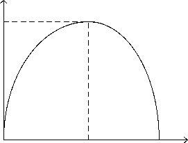
where[·] is still given by (25) . The impact of a change in the tax rate has two opposite effects on the long-run economic growth. Increasing the tax rate relaxed the budegt of each level government to greater expenditures, which increased the output as a result. On the other hand, increasing the tax rate eroded the disposable income of consumers, the gross consumption declined and the output went down. When the tax rate is small, the positive effect is greater, an increasing tax rate drave up the economic growth rate; while the taxation is too heavy, the negative effect is greater, an increasing tax rate drave down the economic growth rate.

The impact of the tax rate on the steady-state growth rate are showed in Fig. 2. When the tax rate decreases till τ <  τ ^∗ , t he steady-state growth rate also decreases; when the tax rate increases till τ >  τ ^∗ , the steady-state growth rate still decreases.

0              τ ^∗ = 1 - β ₁       1 τ

Figure.2. The growth impact of the tax rate

• E.    The Expenditure Structure of the State-level

Government

Expenditures of the state-level government include three parts, productive expenditures, non-productive expenditures and transfer payments to the local-level governments. A change about portions of these parts with total amount constant will have an impact on the growth rate on the balanced growth path.

Holding the portion of transfer payments constant, a change on the portion of productive expenditures results in an relevant opposite change of the portion of nonproductive expenditures. Differentiating both parts of (24) with respect to θ ₁ and evaluating the resulting expression at ∂ G / ∂ θ ₁ = 0 yields

θ1∗ = β2

θ2 ∗ and a steady-state growth rate G∗ satisfying (28) will be

G∗ =β1(1-τ)τ(1-β1)/β1{[•]∗}(1/β1) -ρ(29)

where (29) satisfies

[ • ] ^∗ = ( θ 1 ^∗ φ 1 ) ^{β 2} + ( ^{β 3} θ 1 ^∗ φ 1 ) ^{β 3} + [ ε 1 ( φ 2 + θ 3 φ 1 )] ^{β 4} + [ ε 2 ( φ 2 + θ 3 φ 1 )] ^{β 5} β ₂

Expression (28) means that without change of transfer payments, an optimal ratio between productive expenditures and non-productive expenditures of the state-level government are needed to maximize the steady-state growth rate, which exactly equals to the ratio of their contributions to the output( β2 and β3 respectively). Thence an unique emphasis on productive expenditures or non-productive expenditures will also drive down the long-run economic growth.

• F.    The Expenditure Structure of the Local-level Government

The expenditures of the local-level government are divided into productive and non-productive expenditures under the assumptions of the basic model. Holding total expenditures of the local-level government constant, a change of productive expenditures results in a conrresponding change in non-productive expenditures on the opposite. Differentiating both parts of (24) with respect to ε ₁ and evaluating the resulting expression at ∂ G / ∂ ε ₁ = 0 yields

( ε ₁ ∗ ) (1- β 4 ) _{( ε 2} ∗₎(1- β 5 )

= ^{β 4} ( φ 2 + θ 3 φ 1 )^{( β 4 - β 5)} β ₅

and a steady-state growth rate G ^∗ satisfying (31) will be G = β ₁(1 - τ ) τ ^{(1 - β 1)/ β 1} {[ • ] ^∗ }^{1/ β 1} - ρ (32) where (32) satisfies

[ • ] ^∗ = ( θ 1 φ 1 ) ^{β 2} + ( θ 2 φ 1 ) ^{β 3} + [ ε 1 ^∗ ( φ 2 + θ 3 φ 1 )] ^{β 4} + [ ^{β 5} ( φ 2 + θ 3 φ 1 ) ^{(1 - β 4)} ( ε 1 ^∗ ) ^{(1 - β 4)} ] ^{β 5/(1 - β 5)} β ₄

Expression (31) determined an optimal ratio of productive expenditures and non-productive expenditures of the local-level government. If the left part of (31) is greater, a simply calculation yields ∂ G / ∂ ε ₁ >  0 , which means that under the conditions of a greater portion of productive expenditure of the local-level government, a transfer from the productive expenditure to the nonproductive expenditure will have a positive impact on the output. Sometimes in practice, a short-sighted local-level governmet tends to expense more as productive, e.g. infrastructure, which raised the GDP in a short term but reduces the economic growth rate in a long run. On the contrary, transfering some productive resources to nonproductive expenditures, e.g. local higher education and health care, will pull up the long-run economic growth rate.

• G.    Transfer Payments

Transfer payments are part of the income of the locallevel government and of the expenditures of the statelevel government. Holding total expenditures of the statelevel government constant, a change of transfer payments results in a corresponding change in productive expenditures or non-productive expenditures of the statelevel government. For simplity, we assume that there will be no change in the prortion of non-productive expenditures. Differentiating both parts of (24) with respect to θ ₃ and evaluating the resulting expression at

∂ G / ∂ θ ₃ = 0 yields

θ∗=β4+β5θ∗-φ2

3     β21 and a steady-state growth rate G∗ satisfying (34) will be G = β1(1-τ)τ(1-β1)/β1{[•]∗}1/β1 -ρ(35)

where (35) satisfies

[•]=( θ 1 ^∗ φ 1 ) ^{β 2} +( θ 2 φ 1 ) ^{β 3} +{ ε 1 [ φ 2 +( ^{β 4+ β 5} θ 1 ^∗ - φ ²) φ 1 ]} ^{β 4} +{ ε 2 [ φ 2 +( ^{β 4+ β 5} θ 1 ^∗ - φ ²) φ 1 ]} ^{β 5} β ₂ φ ₁ β ₂ φ ₁

Similarly, expression (34) denoted an optimal ratio of transfer payments and productive expenditures, which is increasing with the contribution of the total expenditures of governments ( β _{4 +} β ₅ ) , decreasing with the contribution of productive expenditures of the state-level government β ₂ and the tax ratio between governments φ ₂ / φ ₁ . That means a greater contribution of the locallevel government to the output absorbs more transfer payments from the state-level government, which implies a higher degree of fiscal decentralization.

• IV.    Extension of the Basic Model: Revenue Atonomy of the Local-level Governments

• A.    Revenue Autonomy

Another type of intergovernmental allocation of public resources concerns revenue assignments. If a local government can raise funds by issuing bonds or borrowing money from banks, that means this local government has the power of ‘revenue autonomy’ rather than a unique tax-sharer. In case of revenue autonomy of the local-level governments, looser budget constraints stimulate local public expenditures, caused a higher degree of fiscal decentralization measured by the expenditure portion of the local-level governments.

• B.    Budget Constraints of Governments

Under similar assumptions of the basic model, in a close economy with only governments and identical economic agents, government expenditures are also supposed to maximize the consumer welfare and divided into those from the state-level government and from the local-level governments, f denoted the former and S the latter. The power of revenue autonomy looses the budget constraints of the local-level governments, that means total government expenditures will be g = f +s= f +s1 +s2 (37) with s1 denotes local government expenditures using taxes shared and s2 denotes those expenditures financed by the local-level governments themselves. We assume that the local-level governments always raise funds as a fixed portion θ ∈ [0,1] of total taxes, and a portion of φ ∈ [0,1] of total taxes goes to the local-level governments gives the budget constraints of governments as f = (1 - φ)τy (38a) s1 = φτy (38b) s2 = θτy (38c)

The maximization problems of governments at two levels are to choose the optimal φ and θ to maximize the social welfare subject to (38a), (38b) and (38c).

• C.    Fiscal Decentralization

Considered revenue autonomy of the local-level governments, the degree of fiscal decentralization could be measured in two ways.

First, we can use the tax-sharing rate between two levels of governments, φ , to denote the degree of fiscal decentralization as in the basic model. While this is indeed a good indicator in practice, question is that this indicator reduces the actual expenditure decentralization to the local-level governments because of its omission of revenue autonomy, particularly when the portion of s 2 in (37) is large, as in some developed countries. However, on conditions of most developing and transitional economies, local governments have strictly limited power on revenue assignments, the tax-sharing rate still operated well.

Another indicator to measure fiscal decentralization degree is the actual expenditure portion of the local-level governments, denoted by

φ ^ˆ = ( φ + θ )/(1 + θ )                   (39)

in our model. This indicator offsets the accuracy question brought by using the tax-sharing rate indicator, reflects the power of the local-level governments under the condition of revenue autonomy. Since it has some problems in practice, such as data gathering, we use this indicator to denote the fiscal decentralization degree in our model is still resonable.

• D.    Description of the Model

In the extension model, an infinitely lived consumer still consumes products and services provided by individuals and governments at a given time to maximize its lifetime utility. An utility function

U ( c , f , s ₁, s ₂)= ^∞ u ( c , f , s ₁, s ₂) e ^{- ρt}dt          (40)

is the lifetime utility of an identical consumer. u ( c , f , s ₁, s ₂) is the similar instantaneous utility fuction of identical consumers and 0 <  ρ < 1 is the discount rate in (40). In a whole lifetime, consumers smooth their consumption in each term through saving and borrowing. When total investment equals to total savings, the steadystate output realized. Similarly, we use

• u ( c , f , s ₁, s ₂) = ln c + ω ₁ ln f + ω ₂ ln( s ₁ + s ₂)      (41)

as the instantaneous utility function in (40). ω_i are nonnegative marginal utility of government expenditures at two levels, i = 1,2 .

For simplicity and without loss of generality, production in the economy is an CES function of capital k and government expenditures as

The problem of an identical onsumer is to choose the optimal consumption bundle to maximize (40) subject to (42) and (43). On the balanced growth path, the economy will grow at the same rate with the consumption, savings and investments. The steady-state economic growth rate, equals to the growth rate of consumption, is a function as

G e = c = a [1 - (1 + 0 ) t ] R ( X ) - p           ⁽⁴⁴⁾

c

R(X) = {a + [p(1 - ф)-Z + у(ф + 0)-Z ](g/k)-Z }-(1+Z)/Z in (44). The same growth rate of the investment and the economy provides a constant government expenditure-capital ratio on the banlanced growth path ,g/k , as g/k = {a/[tz - в(1 — ф)-Z — Y(ф + 0)"Z ]}-1/Z    (45)

Given (44)and (45), the steady-state economic growth rate is simplified as

G . = a [1 - (1 + 0v f - ^Р <1 - « Z - Y^{ф + 0} ‘ Г" ‘ - p ⁽⁴ 6) L ^aT J

A simply expression of (46) considering a Cobb-Doglas production function gives

G . = a [1 - (1 + 0 ) t T ^{( e + Y} )/ ^a (1 - ф ) ^e / ^a ( ф + 0 ) ^Y / ^a -p (47)

• E.    The Growth Impact of Revenue Autonomy

The power of revenue autonomy of the local-level governments enable them to expense more than taxes shared, a higher portion of local government expenditures consequently has impact on the growth rate on the balanced growth path. To see this systemetic effect, we have seen that holding all other parameters in (47) constant, the steady-state growth rate is the function of 0. Differentiating both parts of (47) with respect to 0 yields dg. /a.=awm (48) a(«TZ )( )/Z

W ( X ) = )1 - (1 + 0 ) t ](1 + Z )[ t^z - в (1 - Ф ) - ^Z - Y ( Ф + 0 ) - ^Z ] ^{- 1} Y ( Ф + 0 ) ' ^Z ) - T are satisfied in (48). When z > - 1 and g ₀ >  0 , the right hand of (48) are nonnegative requires that w ( x ) >  0 shoule be satified. Similarly, we consider the simple form of (48) using the CES production function, where w ( x ) >  0 yeilds

₀ <  / О- Т - тф                 (49)

( a + y T

Let 0 * denotes the optimal portion of self-raised funds of the local-level governments, holding other parameters constant, (49) means that

„. Y (1 - t ) - aтф                       ⁽⁵⁰⁾

0 =-----------

(a + Y )t will be satisfied.

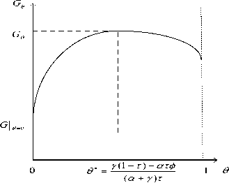
Figure.3. The growth impact of revenue autonomy

When other parameters are constant, expression (50) means that the optimal portion of self-raised funds of the local-level governments is unique. As the power of revenue autonomy of the local-level governments increases till 0 > 0*, a simple caculation of (48) yields 5G /80 < 0 .On the countrary, when the revenue power of 0

the local-level governments are limited till 0 <  0* , 5 G ₀ / 5 0 >  0 . This is called the “Inverted U-shape” relationship between the power of revenue autonomy of the local-level governments and the steady-state economic growth , as showed in Fig. 3.

One point should be noted in Fig. 3 is that when 0 = 0 , the steady-state growth rate remains as that we showed in the basic model as

G| ₀ . 0 = a (1 - t ) t^{( Р + Y} )/ ^a (1 - ф ) ^e / ^a ( ф ) ^Y / ^a - p (51)

• F.    The Growth Impact of the Tax-sharing Rate

In order to study the growth impact of the tax-sharing rate, we started from the relationship between the taxsharing rate ф and the revenue autonomy indicator 0 . The following corollary presents the properties of these two paramters and the steady-state growth rate.

Corollary 1. In a closed economy with two-level governments, holding all other parameters constant, a Cobb-Doglas production function yields:

• b) There is an “Inverted U-shape” relationship between the tax-sharing rate, ф, and the steady-state growth rate, G ₀ .

b) As the expenditure portion of the local-level governments, 0 , increases, the optimal tax-sharing rate , ^ф, should reduces to maximize the steady-state growth rate, G ₀ .

Proof .

• a)    Holding other parameters constant, differentiating both parts of (47) with respect to ф yields:

  5 G ₀ / 5 ф =

  
  

a [1 - (1 + 0 ) t ](1 + Z )( aT ^Z ) ^{- (1 + Z} )/ ^Z [ y ( ф + 0 ) ^{- |1 + Z} ) - в (1 - ф ) ^{- |1 + Z} ) ] (52) ^t^z - в (1 - ф ) ^{- Z} - Y ( ф + 0 )" ^Z ] ^{- 1/ Z}

When Z > -1 and G0 > 0 are all satisfied in (52), the right hand side of (52) is nonnegative requires

Y(ф + 0)-(1+Z) - в(1 - ф)-(1+Z) > 0

A simple caculation of (53) yields

, л r Y 1/(1+Z)z-.x ф + 0 <[Y ]

1 - ф l в J

Inequality function (54) provides a relationship of ф and 0 which is to garuantee a nonnegetive steady-state growth rate. Let ф denotes the optimal tax-sharing rate, inequality function (54) implies

.                Y1'(1 + Z )

ф + 0 | y ।                       (55)

т^ ф^ в J

A simple expression of (55) using a Cobb-Doglas production function is ф= L-Р!            (56)

Р + Y

As the tax-sharing rate increases till φ > φ ^∗ , a simple caculation of (52) yields ∂ _{G θ} / ∂ φ _{< 0} .o n the countrary, when the tax-sharing rate decreases till φ < φ ^∗ , ∂ G _θ / ∂ φ _> 0 . t hat means an “i nverted u- shape ” relationship exits.

• b)    Expression (56) also means that the optimal taxsharing rate, φ ^∗ , is a decreasing function of θ .

This completes the proof of Corollary 1.

The Corollary 1 despribes a general relationship among three variables, φ , θ and G _θ . In order to show these relationship more clearly, we considered numerical simulations.

The parameter configurations considered for the numerical simulations are as follows: α = 0.75 , β = 0.10 , γ = 0.15 , ρ = 0.02 , τ = 0.25 and θ = 0 , 0.20, 0.40, 0.60 and 0.80. The tax-sharing rate ( φ ) and the steady-state growth rate ( G _θ ) are computed as follows. A value of the expenditure portion of the local-level governments ( θ ) are considered for each simulation. For each possible value of the tax-sharing rate φ ∈ [0,1] , the steady-state growth rate G _θ is computed using (36). Once we have this schedule of G _θ , the optimal tax-sharing rate ( φ ^∗ ) is identified as the tax-sharing rate that maximizes the steady-state growth rate and is computed using (56). Fig. 4 shows the simulation results.

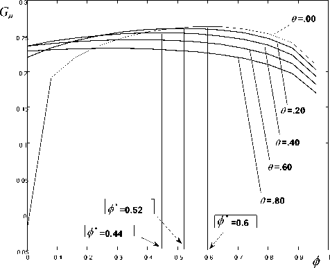
Figure.4. Numerical Simulations

We can see from Fig. 4 that when θ= 0 , an “Inverted U-shape” curve means that the steady-state growth rate (Gθ ) increases as the tax-sharing rate of the local-level governments ( φ) increases, the maximization appears when φ∗ = 0.6 , then goes down. This curve is exactly the one showed in Fig. 3. As the expenditure portion of the local-level governments (θ) starts to increase, the curve becomes smoother, and the optimal tax-sharing rate (φ∗ ) to maximize the steady-state growth rate decreases, equals to 0.52 and 0.44, respectively, when θ = 0.20 and 0.40. Numerical simulations give another proof of Collary.

• G. The Growth Impact of Fiscal Decentralization

Recall that under the conditions that the local-level governments have the power to raise funds by themselves, we use the actual expenditure portion of the local-level governments denoted by (39) as the indicator of fiscal decentralization in our extended model. The above computations, along with Proposition, Corollary and simulations so far, let to the following corollary presenting the properties of fiscal decentralization under the conditions of revenue autonomy.

Corollary 2. In a closed economy with two-level governments and a Cobb-Doglas production function, , holding all other parameters constant, the state-level government chooses the optimal tax-sharing rate( φ ^∗ ) and the local-level governments choose the optimal portion of self-raised funds (θ ^∗ ),

• a)    The optimal fiscal decentralization (φ ^{ˆ ∗} ) yields:

φ ˆ ^∗ = ^γ β + γ

• b)    The relationship between fiscal decentralization and the steady-state growth rate is still an “Inverted U-shape” curve showed in Fig. 2.

Proof .

• a)    Recall that the optimal θ and φ are represented by (50) and (56) respectively, then the optimal fiscal decentralization is identified by (39) will be computed to yield

φ ˆ ∗ ₌ φ ^{∗ + θ ∗} ₌ ^γ               (58)

1 + θ ^∗    β + γ

• b)    If the degree of fiscal decentralization decreases till φ ^ˆ<  φ ^ˆ∗ , that implies φ < φ ^∗ or θ <  θ ^∗ , the steady-state growth rate will increase according to (48) and (52). On the countrary, if the degree of fiscal decentralization increases till φ ^ˆ > φ ^ˆ∗ , that implies φ > φ ^∗ or θ > θ ^∗ , the steady-state growth rate will decrease consequently.

That concludes the proof of Corollary 2.

• V. Conclusions

In our basic model, the relationship of fiscal decentralization and economic growth shows an “Inverted U-shape”. One extension of the model considered intergovernmental transfer payments, productive and non-productive expenditure defference. Comparative static analysis showed that, on the balanced growth path, there was an “Inverted U-shaped” relationship between the tax rate and the long-run economic growth. Optimal ratios between productive and non-productive expenditures of two levels of governments, between transfer payments and other parts of expenditures of the state-level governments are needed to maximize the long-run economic growth.

Other extension of the model considers another intergovernmental allocation of public resources. If the local-level governments have the power of revenue autonomy, the degree of fiscal decentralization should be modified. While we showed that this revenue autonomy does not affect the “Inverted U-shape” relationship between fiscal decentralization and economic growth.