Introduction in quantum optimal control

Author: Ulyanov Sergey, Kovalenko Alexander, Reshetnikov Andrey, Tanaka Takayuki, Reshetnikov Gennadii, Yamafuji Kazuo
Journal: Сетевое научное издание «Системный анализ в науке и образовании» @journal-sanse
Article in issue: 1, 2018.
Free access
This paper describe at the formulation of quantum feedback control theory for continuously observed open quantum systems in a manner that highlights both the similarities and differences between classical and quantum control theory. This paper will involve a discussion of special topics in the field and is meant to provide an overview of current experiments in quantum control.
Quantum control, quantum feedback, optimal control system
Short address: https://sciup.org/14123284
IDR: 14123284
Введение в квантовое оптимальное управление
В этой статье описывается постановка теории квантового управления с обратной связью для непрерывно наблюдаемых открытых квантовых систем таким образом, чтобы выделить как сходства, так и различия между классической и квантовой теорией управления. Работа включает обсуждение специальных тем в этой области и предназначена для представления обзора текущих экспериментов по квантовому управлению.
Text of the scientific article Introduction in quantum optimal control
The purpose of this course is to provide an introduction to the branch of science and mathematics known as control theory, a field that plays a major role in nearly every modern precision device. In the classical engineering world, everything from stereos and computers to chemical manufacturing and aircraft utilizes control theory. In a more natural setting, biological systems, even the smallest single-celled creatures, have evolved intricate, life-sustaining feedback mechanisms in the form of biochemical pathways. In the atomic physics laboratory (closer to home), classical control theory plays a crucial experimental role in stabilizing laser frequencies, temperature, and the length of cavities and interferometers.
The new field of experimental quantum feedback control is beginning to improve certain precision measurements to their fundamental quantum noise limit. New research domain in modern control system theory brought forth together engineers, physicists and applied mathematicians to construct an overview of new challenges that arise when applying constitutive methods of control theory to nano-scale systems whose behavior is manifestly quantum [1-26].
-
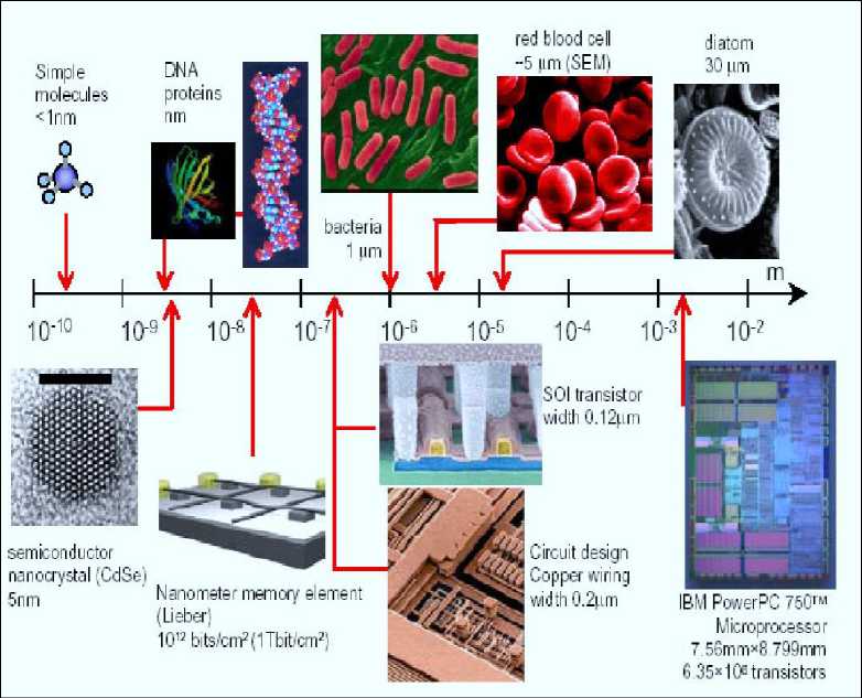
Figure 1 show putting it in scale.
(a)
(b)
Figure 1. Physical local (a) and global (b) size scales
The semiconductor industry was driven by a “smaller-cheaper cheaper-better” synergy model into nanotechnology by aggressive scaling “Moore’s Law” is an integral part of the semiconductor success story. One of the Benchmark in this area is structure design of quantum computer.
-
Figure 2 shows how the physical number of qubits has increased every year.
Several qubits have been demonstrated in solution NMR and in ion/atom traps.
Remark . One- or two- qubit operations have been demonstrated in many solid-state systems within the last two years. In this sense, the twenty-first century is the dawn of the solid-state qubit. It is noteworthy that the slope in Figure 2 shows that the number of bits has increased by nearly 2.7 times over three years, which corresponds to Moore’s law for logic circuits. The increase in solution NMR qubits and ion/atom trap qubits really does fall on this line except for a small shift in the horizontal direction. Although the number of solidstate qubits is too small to agree with the slope, the optimistic expectations of ARDA (10 physical qubits in 2007 and 50 qubits in 2012, and 128 in 2018) do fall on it. This means that quantum computer development is really a rapidly growing field and highly competitive, comparable with that of cutting-edge Si integrated circuits. The goals set by ARDA are ambitious, but they may be attainable through the collective efforts, as example, of NTT Laboratories in cooperation with outside organizations.
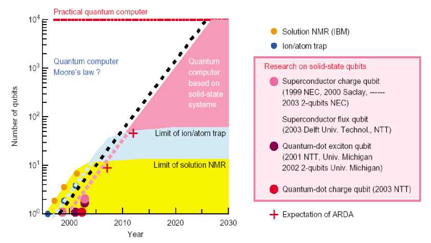
Figure 2. Road map of quantum computers (Only some examples are plotted here)
Remark . On the other hand, a practical quantum computer with about 10,000 qubits will only be demonstrated after 2025, even with this rapid progress. This clearly indicates the need to take a long-term view for quantum computer research. At present, a diverse range of experimental approaches from a variety of scientific disciplines are pursuing different routes to meet the requirements for a scalable quantum computing system. It is too soon to attempt to identify which ones may be successful. This is because the ultimate technology may not have been invented yet. We should remember the history of semiconductor devices where the first successful transistor was made of Ge, but Si is now the established material. Therefore, we need to be careful in comparing different materials, including superconductors and semiconductors. In addition, several qubit gate designs exist. In some electrical and optical manipulations, the quantum logic gate operation is intrinsically limited to operations between nearest-neighbor qubits. This type of logic operation, however, would allow parallel operation within a quantum computer. On the other hand, other approaches are capable of acting as logic gates between widely separated qubits, but they are limited to serial operations. Therefore, for both materials and implementation methods, we should develop various different systems in parallel for the time being.
It was, is and will be a success story for the next decennium of the years to come.
This success story has not yet come to an end but we are approaching increasing challenges to be overcome both scientifically and economically as:
-
• Lithography
-
• Interconnection
-
• Power dissipation
-
• Cost
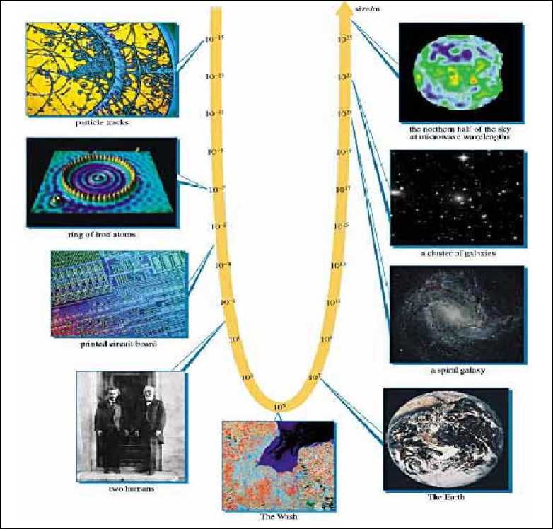
Figure 3 should help to illustrate the scale of things we are entering.
Its primary conclusions were that the number of experimentally accessible quantum control systems is steadily growing (with a variety of motivating applications) that appropriate formal perspectives enable straightforward application of the essential ideas of classical control to quantum systems, and that quantum control motivates extensive study of model classes that have previously received scant consideration.
Figure 3. The scale of things – Nanometers and more
Thus apparently, there are at least two reasons for studying control theory.
First, a detailed knowledge of the subject will allow us to construct high precision devices that accurately perform their intended tasks despite large disturbances from the environment. Certainly, modern electronics and engineering systems would be impossible without control theory. In many physics experiments, a good control system can mean the difference between an experimental apparatus that works most of the time and one that hardly functions at all.
The second reason is potentially even more exciting it is to develop general mathematical tools for describing and understanding dynamical systems. For example, the mathematics that has been developed for engineering applications, such as flying airplanes, is now being used to quantitatively analyze the behavior of complex systems including metabolic biochemical pathways, the internet, chemical reactions, and even fundamental questions in quantum mechanics.
There is substantial interest in extending the concepts from classical control theory to settings governed by quantum mechanics. Quantum control is particularly exciting because it satisfies both of the reasons for studying control theory. First, there is a good motivation for controlling quantum systems. As electronic and mechanical technologies grow ever smaller, we are rapidly approaching the point where quantum effects will need to be addressed; quantum control will probably be necessary in order to implement quantum computation and communication in a robust manner.
On the other hand, control theory provides a new perspective for testing modern theories of quantum measurement, particularly in the setting of continuous observation. Many of the mathematical tools used for analyzing classical dynamical systems can be applied to quantum mechanics in a manner that is complementary to the traditional tools available from physics. The mathematical analysis in control theory has tended to be more rigorous than typical approaches in physics, and quantum control provides a fantastic setting for demonstrating the power of these tools. Modern scientific inquiry and the demands of advancing technology are driving theoretical and experimental research towards control of quantum systems. Compelling applications for quantum control have been noted and have motivated seminal studies in such wide-ranging fields as chemistry, metrology, optical networking and computer science. Experience has so far shown that quantum dynamics and stochastic can be incorporated within the framework of estimation and control theory but give rise to unusual models that have not yet been studied in depth.
The microscopic nature of quantum systems also demands renewed emphasis on accounting for the essentially physical (finite impedance) nature of measurement and feedback interconnections, which limits the applicability of state-feedback formalism and makes quantum filtering an essential methodology for closed-loop control. Open-loop control remains effective in the quantum regime but the actuation terms are generically bilinear. Overall, one begins to see that novel features of quantum systems could spur the growth of a new branch of control theory to develop hand-in-hand with the cutting-edge applications that drive it.
Remark. We should be careful to note that theoretical foundations for quantum control have been in place for some time. Among the participants of our report, Belavkin, Rabitz, Tarn, Krasovski, Samoilenko & Butkovski, Petrov & Ulyanov etc. each reviewed seminal work dating back to the 1980s. But the current resurgence of interest may be attributed to recent advances in experiments on quantum control and to the emergence of high-profile applications in metrology, physical chemistry, quantum information science, molecular spintronics etc.
As example, spintronics is the ability of injecting, manipulating and detecting electron spins into solid state systems. Molecular-electronics investigates the possibility of making electronic devices using organic molecules. Traditionally these two burgeoning areas have lived separate lives, but recently a growing number of experiments have indicated a possible pathway towards their integration. This is the playground for molecular-spintronics, where spin-polarized currents are carried through molecules, and in turn they can affect the state of the molecule. We review the most recent advances in molecular-spintronics. In particular we discuss how a fully quantitative theory for spin-transport in nanostructures can offer fundamental insights into the main factors affecting spin-transport at the molecular level, and can help in designing novel concept devices.
It thus seems appropriate here to emphasize the importance of grounding further theoretical investigations of quantum control in concrete experimental settings and design goals of practical interest. Our intent in writing this report is not to present only a comprehensive review of the field, but rather to attempt to provide a timely piece motivated by presentations given at the different publications that can indicate some points of entry into the recent literature on quantum control and its applications.
We begin with a brief introduction and overview of some compelling applications for quantum control, continue with a survey of relevant experimental systems, and then turn to a more formal presentation of mathematical models and some open problems. For this reason, our course begins with a description of classical systems particularly that of linear feedback control. This is not only practical, since it will allow you to construct servos and controllers for your common laboratory experiments (like locking cavity mirrors and laser frequencies), it is also pedagogical. Understanding the particular details which make quantum systems different from classical systems requires that we first look at classical control theory. Additionally, in our experience, there is a reasonable amount of misconception regarding servos and simple feedback systems in the experimental physics community. In part, most of this is likely due to the fact that one has more interesting problems to deal with when constructing a complicated experimental apparatus. Stabilizing some boring classical detail such as a cavity length in an experiment to do something grand, like generate single photons, is often viewed as a necessary evil. Often, this type of feedback is implemented in a mediocre way rather than with a custom tailored, robust feedback loop.
Remark . In particularly, the purpose of this report is to provide an overview of some aspects of optimal and robust control theory considered relevant to quantum control. The notes begin with classical deterministic optimal control, move through classical stochastic and robust control, and conclude with quantum feedback control. Optimal control theory is a systematic approach to controller design whereby the desired performance objectives are encoded in a cost function, which is subsequently optimized to determine the desired controller. Robust control theory aims to enhance the robustness (ability to withstand, to some extent, uncertainty, errors, etc.) of controller designs by explicitly including uncertainty models in the design process. Some of the material is in continuous time, while other material is written in discrete time. Necessary information from advanced and modern control theory is introduced.
We give an introduction to feedback control in quantum systems, as well as an overview of the variety of applications which have been explored to date. This introductory review is aimed primarily at control theorists unfamiliar with quantum mechanics, but should also be useful to quantum physicists interested in applications of feedback control. We explain how feedback in quantum systems differs from that in traditional classical systems, and how in certain cases the results from modern optimal control theory can be applied directly to quantum systems. In addition to noise reduction and stabilization, an important application of feedback in quantum systems is adaptive measurement, and we discuss the various applications of adaptive measurements. We finish by describing specific examples of the application of feedback control to cooling and state-preparation in nano-electro-mechanical systems (EMS) and single trapped atoms.
While most readers will be familiar with the notion of feedback control, for completeness we begin by defining this term. Feedback control is the process of monitoring a physical system, and using this information as it is being obtained (in real time) to apply forces to the system so as to control its dynamics.
This process, which is depicted in Figure 4, is useful if, for example, the system is subject to noise.
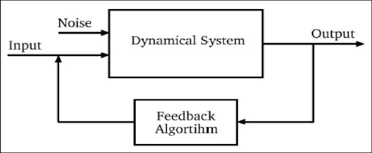
Figure 4. A diagrammatic depiction of the process of feedback control
The output of the noisy dynamical system is monitored. The resulting measured signal is processed by a device which calculates the required input (the feedback) as a functional of this signal. The precise functional used is called the feedback. Since quantum mechanical systems, including those which are continually observed, are dynamical systems, in a broad sense the theory of feedback control developed for classical dynamical systems applies directly to quantum systems.
Remark. Here we use the term classical to refer to systems which are the traditional purview of control theory - mechanical systems obeying Newton’s equations, and electrical systems obeying Maxwell’s equations. However, there are two important caveats to this statement. The first is that most of the exact results which the theory of feedback control provides, especially those regarding the optimality and robustness of control algorithms, apply only to special subclasses of dynamical systems. In particular, most apply to linear systems driven by Gaussian noise. Since observed quantum systems in general obey a nonlinear dynamics, an important question that arises is whether exact results regarding optimal control algorithms can be derived for special classes of quantum systems. The dynamics of an unobserved quantum system is given by Schrödinger’s equation, which is linear. However, the act of continually observing a quantum system will in general induce a non-linear dynamics. In this report we are concentrate our attention on feedback control models. The description role of control object models in optimal control process design is discussed. In addition to the need to derive results regarding optimality which are specific to classes of quantum systems, there is a property that sets feedback control in quantum systems apart from that in other systems. This is the fact that in general the act of measuring a quantum system will alter it. That is, measurement induces dynamics in a quantum system, and this dynamics is noisy as a result of the randomness of the measurement results.
Thus, when considering the design of feedback control algorithms for quantum systems, the design of the algorithm is not independent of the measurement process. In general different ways of measuring the system will introduce different amounts of noise, so that the search for an optimal feedback algorithm must involve an optimization over the manner of measurement. In what follows we will discuss a number of explicit examples of feedback control in a variety of quantum systems, and this will allow us to give specific examples of the dynamics induced by measurement.
Quantum control scenario and applications
A first question that inevitably arises in any introduction of quantum control is: “What makes a control system quantum?” In principle, our current understanding of physics holds that all systems are quantum but manifestly non-classical phenomena are observable only under special laboratory conditions. Roughly speaking, quantum “behavior” emerges in scenarios where a relatively small physical system (with few active dynamical degrees of freedom) can be well isolated from environmental perturbations and dissipative couplings. In some experiments this effectively can be achieved by bringing an experimental apparatus to very low temperatures (as in the superconducting circuit experiments cited below), while in others one can exploit a separation of energy and/or time scales to observe transient quantum behavior at room temperature (as in experiments on atomic ensembles and liquid-state nuclear magnetic resonance - NMR). From a more formal perspective, one could say that quantum mechanics is believed to be a correct microscopic theory of (non-relativistic) physics but that the reduced dynamics of subsystems nearly always corresponds closely to models that fall within the domain of classical mechanics. Hence strongly non-classical behavior can only be observed in a subsystem on timescales that are short compared to those that characterize its couplings to its environment (see, Figure 5 and 6).
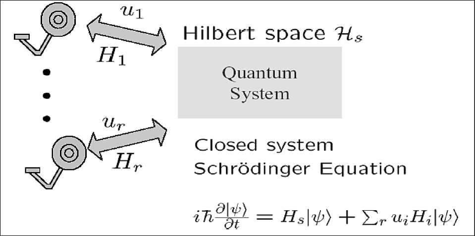
Figure 5. Closed quantum system
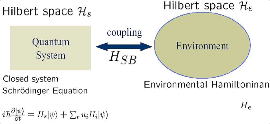
Figure 6. Open quantum system
A quantum system is described by its corresponding Schrödinger’s equation. The Schrödinger’s equation for a quantum control system
-
8 ^( X, t ) = [ H 0 ( t, X ) + и ( t ) Hi ( t, X ) ] ^ ( X, t )
,
where H is the free Hamiltonian (energy) of the system; H is the interaction Hamiltonian of the system while being coupled to the control apparatus in the semiclassical treatment; ^ ( x , t ) is the state of the system. Open loop quantum control system is considered as a single larger system in an augmented state space “System + Environment = Hs ® HA.” A quantum system interacting with a thermal bath is called an “open” quantum system.
Open quantum systems lose their coherence or superposition in the order of a few microseconds to milliseconds depending on the interaction. An open quantum system can be described as follows (see, Figure 7).
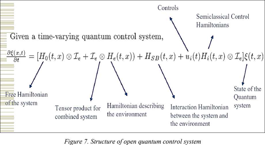
Figure 8 show structure of quantum control systems for described cases.
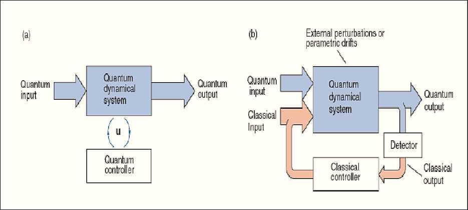
Figure 8. Structures of open-loop (a) and closed-loop (b) quantum control systems
In the case of any macroscopic object, such as an ordinary mechanical pendulum, there are so many such couplings (e.g. via mechanical coupling to its support and to air molecules) that these timescales are inaccessibly short. From an even more abstract perspective, one could say that Schrödinger’s equation is meant to apply to the universe as a whole (whose ‘internal’ degrees of freedom are densely interconnected) while physical experiments deal only with embedded subsystems. Unless great care is taken to suppress the environmental couplings of an experimental system, the overwhelming tendency is for its behavior to appear classical, or at least imperfectly quantum.
The accurate quantitative modeling of “imperfectly quantum” behavior in open systems (i.e. those with non-negligible residual environmental couplings) is a subject of intense study in many branches of physics. Generally speaking, one finds fundamental theory in the fields of quantum statistical mechanics and mathematical physics, with more system-specific results in fields such as atomic physics, quantum optics and condensed matter physics. One of the main goals for theoretical research in quantum control will be further to integrate what is known from the physics of open quantum systems with core engineering methodologies.
A second question that may naturally arise at this point is: “Why should we study quantum control?” One answer is that the abovementioned integration of the theory of open quantum systems with estimation and control appears to provide an important new conceptual framework for the interpretation of quantum mechanics itself. By scrutinizing quantum mechanics as a theory for the design of devices and systems, as opposed to a theory for scientific explanation only, we gain new insight into obscure features of quantum theory such as “ complex probability amplitudes ” and “ collapse of the wave function .” In particular, we are able to make more focused comparisons between classical and quantum probability theories. But a second compelling answer to the question at hand is that various branches of research on nanotechnology are advancing to the point of investigating “mesoscopic” devices whose behavior remains quantum on timescales of functional relevance. It thus seems clear that in order fully to exploit the powerful methodologies of control theory in the design and implementation of advanced nano-scale technologies control theory needs to be reconciled with quantum mechanics.
The defining characteristic of a quantum system, from the perspective of control theory, is as mentioned above that measurement causes its state to change. This property is referred to as backaction, an inevitable consequence of the Heisenberg uncertainty principle. In the classical world, it is (in principle) possible to perform a non-invasive measurement of the system as part of the control process. The controller continuously adjusts the system dynamics based on the outcome of these non-invasive measurements. However, in quantum mechanics, the very act of observation causes the state of the system to wander even farther away from the control target. In this sense, the effect of backaction is to introduce a type of quantum noise into the measurement of the system's state. Fortunately, it is possible to think of quantum control in a context that is similar to classical control, but with additional noise source due to the measurement backaction. Therefore, it is theoretically possible to adapt existing control knowledge to make it apply in quantum settings, although there are some mathematical surprises since (unlike classical dynamics) continuous observation of quantum systems prevents them from achieving steady-state.
As we hope the following discussion will illustrate, this reconciliation does not appear to require any radical reformulation of control theory. It does however seem that nanoscale systems (broadly defined) and quantum control present new classes of models that fit within the scope of traditional analysis and synthesis methods but have yet to be studied in depth. To date there have been a number of publications that demonstrate the use of standard control-theoretic techniques to analyses models of quantum-physical origin; we will attempt to review briefly them here. We prefer to emphasize the recent development of concrete applications tied to experimental research that generate urgent questions most naturally addressed by quantum extensions of estimation and control theory. These applications and questions are in turn motivating the thorough and principled development of certain practical aspects of quantum control.
A first major application area, to be described in greater detail below, is protein structure determination via nuclear magnetic resonance (NMR). Ideas from control theory have clear relevance to this field because protein structure determination can naturally be viewed as a problem in system identification. In the typical setting one has foreknowledge of the types of atomic nuclei that constitute a given protein, and has experimental tools that can induce rotations of these individual nuclei and collect signals that gauge their precise response to applied controls.
Proteins can be redesigned to fold downhill on a free energy surface characterized by only a few coordinates, confirming a principal prediction of the ‘energy-landscape’ model. Nonetheless, natural proteins have small but significant barriers. Spectroscopy and kinetics reveal potential biological causes for activation barriers during protein folding: evolution against protein aggregation and for protein function. Thermodynamically favored reactions of small organic molecules, such as combustion, are generally quite slow at room temperature. They must proceed over large activation barriers during bond-breaking and -making.
Protein folding is generally much less favored thermodynamically (protein function often requires proteins to be flexible and at the brink of stability), yet folding is fast at room temperature. In the test tube, denatured states of natural proteins last only for milliseconds to hours under conditions favorable for folding, in contrast to the long shelf life of organic compounds. The high speed of protein folding, compared to most barrier-controlled chemical reactions, is due to the near-cancellation of enthalpic and entropic contributions to the free energy during the folding process. Proteins can make energy-lowering contacts and become compact in small steps, so no large mismatch appears en route to the folded product. Small barriers in the free energy of folding are distributed along several reaction coordinates, rather than being lumped into one local high-energy barrier. Energy-landscape theory, a statistical-mechanical treatment of protein folding, predicts that this cancellation could be nearly perfect. Such proteins would fold downhill in free energy, on timescales as short as about 0.5 µs for a bundle of three helices.
Landscape theory makes a key prediction that can be tested by very fast folding of engineered proteins: that the entropy and enthalpy contributions can cancel under ideal folding conditions (see, in details below Figure 9).
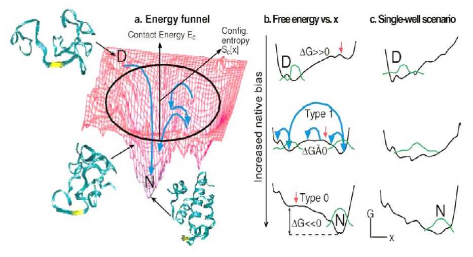
Figure 9. (a) Energy or enthalpy funnel, with λ unfolded conformation at high energy, compact globule at moderate energy, and native state at low energy. (b) Free energy plots reduced to 1 reaction coordinate (2–5 are probably needed for a realistic description of folding). (c) Single-well downhill folding scenario at all biases towards the native state
Remark. The radial coordinate is proportional to the logarithm of the number of protein conformations at a given energy (the configurational entropy, which is higher at higher energy). The angular coordinate symbolizes the many other folding coordinates. The bias towards the native state increases from the top to the bottom. The middle plot corresponds to most natural proteins (type-1 or barrier-limited folding, the green protein population is split into two states). The bottom plot corresponds to the extreme native bias possible with engineered proteins under highly stabilizing solvent conditions (type-0 or downhill folding). The large blue arrow corresponds to slow, exponential type-1 folding; the small blue arrows correspond to fast diffusive motions that lead to type-0 folding. Note that the free energy surface retains roughness even in the downhill case, caused by unavoidable frustration of folding by the finite amino acid alphabet and physical constraints. Unlike (b), in this case strong deviations from cooperative thermodynamics are expected.
In Figure 9, when all stresses against folding (denaturants, ‘bad’ side chains, high temperature, etc.) are removed, the protein folds ‘downhill’ without any barriers greater than 1–2RT (‘type-0’ folding scenario).
Another prediction of the energy-landscape model is that different rates are obtained by different spectroscopic probes during downhill folding. This is illustrated in Figure 10.
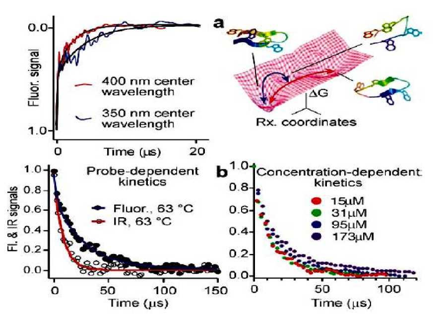
Figure 10. Proteins or peptides folding on a rough downhill free energy surface do not have a single well-defined rate. (a) Difference in relaxation rates observed for the beta hairpin peptide trpzip2 at two different fluorescence wavelengths, and two possible paths on the free energy surface with structures computed by molecular dynamics; (b) Infrared and fluorescence spectroscopy yield different folding/unfolding kinetics for the helix bundle λ Q33Y mutant at 630C , and kinetics of the λ D14A mutant are aggregationdependent above 30-µmol concentration
Slower folding mutants, which fold over an activation barrier, show neither a wavelength dependence nor transient aggregation below 200 µmol. When there is a barrier, protein populations are small in the region along x where probes such as infrared, circular dichroism, fluorescence, or NMR spectroscopy switch from their denatured to their native signatures. Thus the observed signals are a linear combination of only the folded and unfolded state signals, and they are probe independent. When landscape roughness is the only barrier left, kinetics are no longer homogeneous, and different results are observed with different probes. This has been confirmed for peptides whose free energy surface computed by MD is rough and flat, as well as for designed downhill folders. When there is no substantial barrier in the energy landscape, the residual ‘roughness’ can be quantified directly.
The unknown parameters of the system are the relative spatial positions of the various nuclei, which can be inferred from experiment by estimating the relative strengths of the dynamical couplings among nuclei.
Questions of optimal procedure arise because measurement signal-to-noise ratios are typically quite low, because dissipative mechanisms suppress the observability of dynamical couplings among the nuclei, and because the total number of measurements that must be made to establish the structure of a protein is tremendously large (thus putting a premium on speed of the identification procedure). It is intriguing to note that, even though NMR researchers have been working for many decades to optimize relevant techniques, the recent introduction of control theoretic methods has enabled some substantial improvements in performance (with high practical impact). Many further opportunities can be identified for the application of control theory to NMR.
Over the past decade, a number of groups have proposed and demonstrated close connections between magnetic resonance (of nuclear and/or electronic spins) and quantum information processing. The quantum states of nuclei in certain types of molecules and solid-state systems can be well shielded from environmental perturbations, making them an attractive physical locus for the storage and processing of 13
quantum information. Manipulation of individual nuclear states and conditional transformations of the state of one nucleus based on that of another (corresponding to the implementation of a quantum logic gate) can be accomplished via tailored radio-frequency (rf) electromagnetic fields. In this context questions of optimal control arise for much the same reasons as in protein structure determination, with the additional consideration that large-scale quantum computation may require extremely high fidelity (with inaccuracy € 10 - 4 ) in these elementary quantum state transformations. This need for high fidelity can be compounded by the fact that in real experiments it is typically necessary (especially in NMR) to work with a sample containing very many identical molecules, in order to make the ‘readout’ signals sufficiently strong that they can be detected above instrumental noise. The unavoidable presence of inhomogeneities across such a large sample of molecules then demands a certain degree of robustness in the control policies employed, generating further interesting challenges for the theory.
Similar quantum control problems arise in a wide range of physical implementations of quantum information processing. In systems from atomic physics, the nature of the problems is very similar to what has been described above for the setting of magnetic resonance. In solid state systems one generally finds an intriguing combination of issues of both identification and control. Whereas accurate ab initio models can often be constructed for NMR and atomic systems, the modeling of solid state systems typically requires a more phenomenological approach. In particular, it is seldom possible to derive accurate models for the residual environmental couplings of something like a superconducting quantum circuit. The precise nature and strength of these couplings should be known in order to design control schemes that maximize the fidelity of elementary quantum operations, which as discussed above should be very close to perfect if one is ultimately interested in large-scale quantum computation. Some recent theoretical research has also shown that tools from control and dynamical systems theory can play a substantial role in the formulation and analysis of fault-tolerant architectures for quantum computation and communication.
Quantum computation represents a very high-profile long term goal in nano-scale science and technology; the related field of quantum metrology (or quantum precision measurement) provides a setting with similar technical challenges and with near-term payoffs for the exploitation of quantum control. In applications of high strategic and industrial interest, such as prompt and accurate estimation of magnetic fields, electrical currents, time delays, gravitational gradients, accelerations and rotations, it is just now becoming possible to construct laboratory prototype systems whose leading-edge performance is enabled by techniques that exploit quantum coherence and is limited by noises or uncertainties of quantum-mechanical origin. In these contexts it is natural to look to quantum control to provide techniques for achieving robust performance, based on approaches such as optimal design, adaptation and real-time feedback. Preliminary studies grounded in several different experimental settings have shown, e.g. that real-time feedback can be used to preserve quantum-limited sensitivity gains in the presence of multiplicative uncertainties that would otherwise nullify them. Concrete targets for the application of such methodology range from atom interferometer-based inertial sensing systems to grand scientific projects such as the Laser Interferometer Gravitational Wave Observatory (LIGO). In both of these examples, promising strategies exploiting quantum phenomena have been formulated to surpass near-term performance limits, but quantum control techniques will likely be required in order to implement them robustly.
The final application area we wish to highlight is control and identification of chemical reactions. As has been discussed in some excellent recent review articles, tailored laser pulses can be used to induce and to steer molecular processes ranging from fragmentation to electron transfer and high-harmonic generation. It has been noted that the typically complex nature of the interaction between applied fields and intrinsic dynamics in an optimal control solution could make it possible to design highly selective and sensitive approaches to detecting dangerous chemicals in an environmental monitoring scenario. An interesting feature of recent work on control of chemical reactions is that highly successful control solutions have been “discovered” using learning loops that combine computer optimization algorithms with fast and automated laboratory apparatus for experimentally (as opposed to computationally) evaluating the performance of trial solutions. Such an approach is particularly powerful in the chemical reaction setting as it is often infeasible to obtain accurate models for the relevant molecular dynamics. Early experimental successes have provided strong motivation for theoretical research on improved learning algorithms and on methods for “inverting” the empirically-optimized control solutions to infer pertinent properties of the molecular dynamics.
Looking across these applications some common theoretical themes and challenges emerge. Many experiments, such as those in NMR, involve the simultaneous manipulation of an ensemble of systems with non-negligible dispersion in important physical parameters. The control challenge is to find excitations that are robust to such inhomogeneities. These problems naturally motivate a class of infinite-dimensional systems that are highly under-actuated, as one is trying to steer a continuum of systems using the same control.
Such models raise interesting controllability issues that are discussed in this report.
Remark . Optimal control problems also arise naturally for quantum systems. Generally speaking, controls that achieve their objective in minimum time are desired to minimize dissipative effects associated with residual couplings to the system’s environment. From a mathematical perspective, many of these problems reduce to time-optimal control of bilinear systems evolving on finite or infinite dimensional Lie groups. Although bilinear control problems have previously been studied in great detail, rich new mathematical structures can be found in quantum problems. The added structure enables complete characterization of time-optimal trajectories and reachable sets for some of these systems, as described below. Another class of quantum optimal control problem is steering in the presence of relaxation. Recent work of this type has shown, e.g. that significant improvements can be made in the sensitivity of multidimensional NMR experiments. We now present examples of feedback control applied to three specific quantum systems.
The field of quantum molecular control
Prior to the recognition of the laser field design problem as a control problem, physicists and physical chemists had attempted to design laser fields based on physical intuition. However, due to the complex dynamics of molecules which are most accurately modeled by the Schrödinger equation, it is difficult (if not impossible) to arrive at intuitive field designs that will achieve the desired objective. By 1985 little progress had been made on the field design process. This problem can be recognized as a control problem and to formulate the quantum molecular control problem as an optimal control problem, to explore issues of existence of controllers, and to validate the field designs by means of numerical experiments.
We can plagued by the fact that the bilinearity of the control problem, which is legislated by the way in which the laser field acts on the state in the Schrödinger equation, ruled out the possibility of exploiting the results of linear systems theory - which by that time had reached a high level of maturity and sophistication. In addition, having the instincts of a control engineer, we alarmed that the only control fields that could be envisaged at the time were of the open loop variety - given that the desired molecular dynamics was expected to be complete in hundreds of femtoseconds while observation and feedback on this time-scale was impossible. Having ruled out the possibility of feedback design, we can to investigate the possibility of designing open loop controllers that are robust to uncertainties in the molecular Hamiltonian and to perturbations in initial conditions.
Remark. Molecular control . Since the beginning of alchemy one of the primary goals of chemists has been to stimulate chemical reactions to form desired products. Traditionally these stimuli were applied by changing the global thermodynamic variables such as the temperature and the pressure or by adding the appropriate combination of reagents to achieve desired products. In stimulating such chemical reactions it often happens, that only a certain fraction of the reagents combine to form the desired products while the remaining reagents may combine to form a number of unwanted byproducts. In addition, there are products that cannot be produced by varying such global control variables. It is, therefore, desirable to search for alternative, more selective, and perhaps more efficient ways to stimulate chemical reactions. Neighboring atoms within molecules frequently have net opposite charges on them (the water molecule is a typical example), and the dipoles formed by such pairs of atoms act as microscopic “handles” on the molecules. Using applied electric fields it is possible to try to excite the molecules in a desired way. Another possible way to effect chemical reactions is to use stimulated molecular emission to prepare large quantities of molecules in selected states which are inaccessible by simple absorption. Although these new modes of stimuli offer the possibility of more selective excitation, their success depends on being able to determine the correct field to apply in order to achieve the desired objective.
Remark : Design by intuition The idea of using electric or optical fields to achieve selective chemistry was not new. Indeed, a great deal of research in this area had been done over the previous thirty years. Unfortunately, prior to the application of control theory, the field designs, which were often based on intuition, were largely unsuccessful. For example, if there was a need to break a particular bond within a 15
molecule, then simple intuition would indicate that excitation at the frequency associated with that bond could induce a resonance which would ultimately break the bond. However, due to the coupling between the bond in question and the remainder of the molecule, it is extremely difficult to localize the energy imparted to the molecule within the bond. It is clear that the complicated dynamics and interference structure of the molecule have to be incorporated and perhaps even exploited in the field-design process. These initial attempts were largely unsuccessful in all but the simplest of objectives. Indeed, inspection of the complex structure of the required laser field designs, constructed using control theory, clearly illustrate the limitations of the intuitive field designs - akin to attempting to play a complicated piano concerto with a single finger.
Two model systems
We continue this introductory section with the brief mathematical description of two quantum systems which arise often in applications of quantum control ideas. The first one is the one-half spin particle which is the quantum system with the state space of smallest dimension, namely C2 . Spin one-half systems and two-state systems in general are referred to as qubits in the Quantum Information literature and form the building block of many proposed Quantum Computation and Communication technologies. This makes the study of these systems very important. The other system we will briefly describe is the so-called Morse oscillator. This is the quantum version of a mechanical oscillator with non-linear restoring force that models the force between two atoms in a molecule. In other words, it is a quantum mechanical model of a chemical bond.
Example: The spin- У2 particle . Spin is a purely quantum mechanical degree of freedom with no classical counterpart. It corresponds to an “internal” angular momentum of the particle. Like a rotating particle with charge has a magnetic dipole moment proportional to its angular momentum, so does a particle with spin. In some sense, the spin is an elementary inherent magnetization of particles. Spin interacts with magnetic fields, possibly created by other spins. The electron, the proton, the neutron and many composite nuclei have spin- ^ . This is the simplest of all quantum mechanical systems.
The state space is C2 and the Hamiltonian is H = —Y ^ SiBi , where Bx, By, Bz are the components i=x, y, z of the magnetic field at the position of the particle and Sx, Sy, Sz are the spin operators. They are self-adjoint operators in C2, so they are 2 x 2 Hermitian matrices.
They are simply expressed in terms of the Pauli matrices,
^ x
( 011
1)
07
^ .
( 0 -i)v i 0 ,
(1 0 )V0 17
as S; = — o^. y is a property of the particle called the gyromagnetic ratio, and it may be positive or negative. Here, we take y > 0. In most applications, one applies a large uniform, constant magnetic field Bo in one direction (say z). The reason for this is to overpower any random magnetic fields in the locality of the particle. One then applies uniform time-dependent fields in the x and/or y directions that act as controls. The dynamical equation has the form
id^ = 1 Y kaB + GxBx ( t ) + ^yBy (t )}^ . (1)
This equation can be rendered dimensionless by defining the variables
®0 = Y B0, T = ^01,
B By
u, = , uv = ~ x B0 y B0
,
й)0 is sometimes referred to as the Larmor’s frequency of the spin. The control system takes the simple form
. dw
i
dT
—
1 (
^z + ^xU + ^yuy
^V,
w e C2 V
It is controllable with either control input ( u or u ).
Example: The Morse oscillator. This infinite dimensional system is a model for the vibrational dynamics of two-atom molecules. Its state space is
L (R)
. The Hamiltonian operator is
Hо =
2 d 2
2m dr2
+ U ( r)
with the Morse potential
U (r ) = Uо
exp [—a( r — r0 )] — l}2 — 1
Figure 11 shows the Morse potential, where r is the intermolecular distance, m is the reduced mass of the molecule and r the equilibrium distance of the molecule. a determines the width of the molecular well and V its depth.
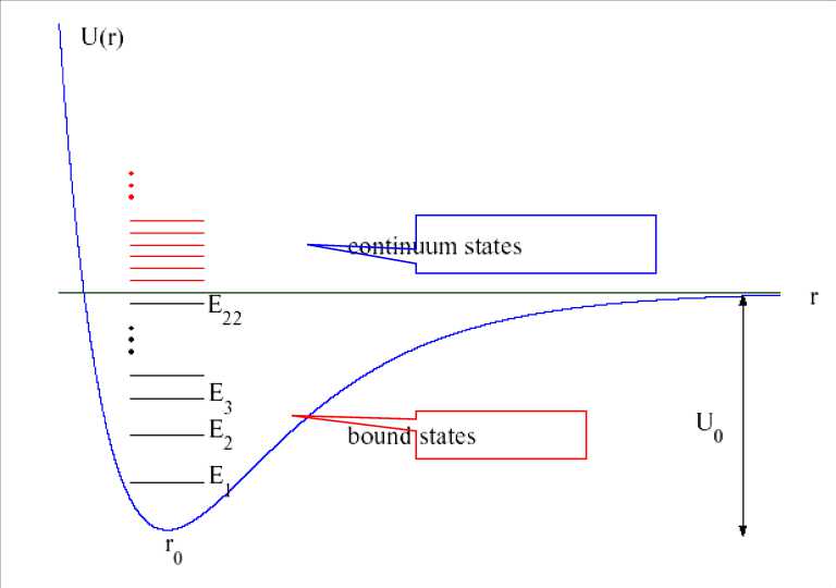
Figure 11: The Morse potential for the OH bond
The spectrum of the Hamiltonian operator contains a set of discrete points as well as a continuum.
The discrete energy eigenvalues are given by the expression En =
Й 2 a2
■ v2mv
2m
h a
- n
-
1
2
, where
n = 0,
V —1
h a 2
. Every E > 0 belongs to the continuous part of the spectrum. The discrete energy
levels correspond to bound states of the molecular oscillation while the continuous energies correspond to unbounded (relative) motion of the two atoms.
Thus, a transition of the molecule from a bound state to a state in the continuum represents the breaking of the molecular bond. This phenomenon is called the dissociation of the molecule and is very important to Quantum Chemistry.
Indeed, the role of the laser as a chemical catalyst is exactly that, to break existing bonds, so that new ones may be formed. The interaction of the molecule with the electric field u of a laser is modeled by the interaction Hamiltonian (in the electric dipole approximation): V nt( t ) = — д ( r ) u ( t ) , and ц ( r ) is the molecular dipole function. A common form for it is ^ ( r ) = ^ r exp | — Г | , ( ^ and r0 are parameters of
V r )
the interaction). In the following, for the purpose of specific examples, we use the model of the OH bond which has 22 bound states.
The optimal control formulation
By 1985 the field of molecular control was ripe for the introduction of techniques from systems theory. The contribution was vital to the introduction of the optimal control formalism in the field of molecular control. In this section we will outline the initial formulation that was used in 1988. Let the spatial domain be Qe R n and consider control on a finite time horizon [0 , T]. Let X = L2 ( Q ) , Xt = L 2 ( Q , [ 0, T ] ) and XHS is the Hilbert Space of Hilbert-Schmidt Operators.
The optimal control problem is prescribed by minimizing the following cost functional:
T
J [U ] = ^ (Q T )—w (□), Q (w (Q T)—w (O^^+fU, U^ds subject to the dynamics of the Schrödinger equation with a molecular Hamiltonian H :
d^ = — i- (H0 + U)y, with V (x,0) = Wo (x) dt over all U e XHs. Here W e X is a specified reference state to which we wish to push the final wave function w ( x, T ), and Ho =-—V + Vo, and Uw = f u ( x, x, t W (x , t) dx . Introducing the Lagrange multiplier function a (x, t) we minimize the Lagrangian:
L[U;w,a] = J[U] + Re< Jja[w + i(H + U)w) 0 Q V )
0 Q
*
> dxdt
where ( ) denotes the complex conjugate. By taking Frechet derivatives of L [ U ; w , a ] with respect to a , w , and U we obtain the following necessary conditions for a minimum:
IVP:^^ = -—(Ho + U)y with У(x,0) = Уо(x) dt 00
FVP: — = - — (Ho + U)a with a(x,T) = 2{у(x)-у (x,T)} dt
Gradient : 0
T
= J J 2ви - Re I a - у0 £V V
SUdxdt
The initial-final value problems (5) form the basis for a numerical gradient numerical search procedure to locate a minimum. A monotonically convergent algorithm due to Krotov is typically used to search for a minimum.
By exploiting the lower semi continuity of the norm, the weak closure of the unit ball in L , and the regularity of the solution it is possible to prove the following theorem (see, see in details below):
Result 1: There exists a solution U e L ( XH ; [ [ 0, T ] ) and a corresponding у e Xt that solves the optimization problem.
Example . In the following example we wish demonstrate the control design process for a simple diatomic molecule in which the molecular potential is assumed to be given by the Morse potential from Eq. (4): V ( x ) = D ( 1 - e - y ( x " x 0 ) ) 2 .
It is assumed /i = 1, m = 2, D = 10, у = 1/ ^J10, T = 18 and that the initial wave packet is a Gaussian of unit width centered at x0 = 6 and that the target wave packet is a Gaussian having the same shape but centered at x = 8, i.e.:
1 _1 ।
( x - x ') 2 ) 2 l2
у (x,0) = g (x,6,1) and у (x, T) = g (x,8,1), where g (x, xf, l ) = n 41 2 exp
V
In this experiment the laser field was of the form u ( x, t ) = E ( t ) B ( x ) = E ( t )( x – x( 0)) so that the dipole moment function B(x) is assumed to be linear.
In Figure 12 we provide a space-time contour plot of the probability density of the wave packet У (x, t)| juxtaposed with the corresponding electric field E(t). We observe the complex structure of the field E (t) as well as the corresponding dynamics of the wave packet as it makes its way to the target state.
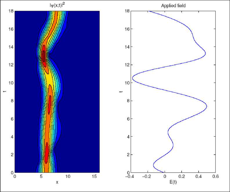
Figure 12: A space-time contour plot of the probability density of the wave packet juxtaposed with the corresponding electric field
In Figure 13 we provide a 3D plot of the same probability function which is close to the target Gaussian at time T = 18 .
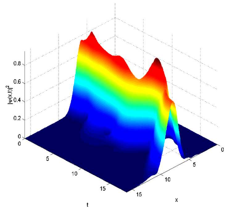
Figure 13. 3D plot of the probability function which is close to the target Gaussian at time T = 18
This formalism was adopted by many subsequent researchers as they endeavored to design fields to control more complex molecules. Many researchers also used this initial optimal control framework to explore molecular control using semiclassical and even classical molecular models. In principle, this formalism should be adequate to design laser fields for molecules containing any number of atoms. Unfortunately, the number of space dimensions n required in the solution of the Schrödinger equation grows with the number of atoms in a molecule.
Thus field designs are severely limited by the computing resources required to solve the initial and final value problems.
Uncertainty and robust control design
Due to the fact that the molecular Hamiltonians for large complex molecules are not known precisely there are likely to be considerable uncertainties in the molecular models used in the design process. Because of these uncertainties and the restriction to open-loop controllers, it was a strong protagonist for establishing a robust design methodology. In this section we briefly outline the extension of the previous optimal control framework to achieve robust field designs. One drawback of the optimal design approach used in the work described above is that these controllers are likely to be sensitive to uncertainties in the molecular Hamiltonian and in the initial state of the system. In order to achieve more robust field designs, averaged cost functionals corresponding to those described in the previous section have been considered.
In particular the optimal control problem involves minimizing the following cost functional:
T
J U ]=E„.. [(v (a T) - V (a) ■ Q ( v (a T) - V (□})) , ]+eJ U, Uhs ds
¥ = - i- ( H 0 ( x ) + E ( t ) B ( z ) ) ^ , with ¥ ( x ,0 ) = ¥ 0 ( x ) subject to: dt .
Here E [□] represents the expectation operator. It is possible to define a family of cost propagator x , т 0
operators which make it possible to perform explicit averaging of the cost functionals. These averaged cost functionals do indeed lead to field designs that are demonstrably less sensitive to perturbations in initial conditions or to fluctuations in the parameters of the molecular Hamiltonian.
Controlling nanoscopic systems
The first is a nano-mechanical resonator, and the second is a single atom trapped in an optical cavity. In both cases the goal of the feedback algorithm will be to reduce the entropy of the system and prepare it in its ground state. A nano-mechanical resonator is a thin, fairly ridged bridge, perhaps 200 nm wide and a few microns long. Such a bridge is formed on a layered wafer by etching out the layer beneath. If one places a conducting strip along the bridge and passes a current through it, the bridge can be made to vibrate like a guitar string by driving it with a magnetic field. So long as the amplitude of the oscillation is relatively small, the dynamics is essentially that of a harmonic oscillator. One of the primary goals of research in this area is to observe quantum behavior in these oscillators. The first step in such a process is to reduce the thermal noise which the oscillator is subject to in order to bring it close to its ground state. Typical nano-mechanical resonators have frequencies of the order of tens of megahertz. This means that to cool the resonator so that its average energy corresponds to its first excited state requires a temperature of a few milliKelvin. Dilution refrigerators can obtain temperatures of a few hundred milliKelvin, but to reduce the temperature further requires something else. It was shown that, at least in theory, feedback control could be used to obtain the required temperatures.
To perform feedback control one must have a means of monitoring the position of the resonator and applying a feedback force. The position can be monitored using a single electron transistor, and this has recently been achieved experimentally. A feedback force can be applied by varying the voltage on a gate placed adjacent to the resonator. Quantum electromechanical systems are nano-to-micrometer (micron) scale mechanical resonators coupled to electronic devices of comparable dimensions, such that the mechanical resonator behaves in a manifestly quantum manner. We outline several possible schemes to demonstrate various other quantum effects in (sub)micron mechanical resonators, including single phonon detection, quantum squeezed states and quantum tunneling of mechanical degrees of freedom. Thus quantum electromechanical systems (or QEMS for short) are an emerging branch of mesoscopic physics made possible by recent advances in microfabrication technology.
A QEM device typically comprises a nano-to-micron scale mechanical resonator, such as a cantilever (suspended beam which is clamped at one end) or bridge (suspended beam clamped at both ends), which is electrostatically coupled to an electronic device of comparable dimensions, such as a single electron transistor (SET). While a mechanical resonator comprises three times as many normal vibrational modes as it does atoms, only the lowest, few flexural modes will strongly couple to the electronic device. Provided that the quality factors of these lowest modes are very large, then for small amplitudes the mechanical resonator behaves electively like a few independent damped harmonic oscillators. The quality factor for a given oscillator is defined as Q = гот , where ro is the oscillator angular frequency and т is the energy decay time constant, i.e., the time taken for the energy stored in the oscillator to decay by a factor e from its initial value. Measured quality factors of the lowest modes of nano-to-micron scale mechanical resonators in moderate vacuum are typically in the range 10 3 - 10 4 . With the appropriate temperature and vacuum conditions, and device operating parameters, these oscillators will behave in a manifestly quantum manner, as indirectly evidenced through the electronic device behavior.
Let us consider quantum limits of the resonator. An important rule-of-thumb for observing quantum behavior is Vm %kBT, where vm is the resonator’s lowest, flexural fundamental mode frequency (the “m” subscript denotes “mechanical”), T is the resonator temperature and and k are Planck’s and Boltzmann’s constants, respectively. The lowest, typical achievable temperature using a dilution refrigerator is about 30 mK which gives vm %d600 MHz , in the radio frequency regime. For the example of a cantilever with length l, width w, thickness t, mass density p and Young’s modulus E, the frequency v is v = 0.56 — ----.
mm l z\12 p
Assuming, for example, the bulk material values for silicon (Si): E = 1.5 x 10¹¹ Nm-2 and p = 2.33x10³ kg m 3, and expressing the size dimensions in microns and frequency in GHz, vw becomes
V = 1.3 p-. For example, a 1 pm long and 0.1 pm thick Si cantilever has a fundamental frequency of 130
MHz.
Thus, to observe quantum effects, submicron scale mechanical resonators must be employed. Note, however, as we shall learn in this review, condition /z vm %kBT is not always strictly necessary in order to observe quantum behavior. For example, it should be possible to demonstrate quantum entanglement at T = 30 mK for a resonator with vw = 50 MHz . Decoherence due to the interaction of the resonator with its environment governs the quantum-classical border in this case. Nevertheless, the lower temperature limits to which mechanical resonators can be cooled essentially define the size scale for which quantum elects can be observed; it is therefore extremely important to develop alternative methods of cooling suited to mechanical devices if quantum e1ects are to be demonstrated at larger-than-micron scales.
Despite the relatively small sizes of the (sub)-micron-scale mechanical devices, they comprise up to □ 1010 - 1011 atoms and so in some sense their quantum behavior would be deemed macroscopic, certainly substantially pushing the quantum-classical divide out of the microscopic and into the macroscopic realm for mechanical systems.
Another important quantum mechanical scale is the zero-point displacement uncertainty in the m fundamental mode, which for the cantilever is Ax = --------, where m.f = — is the cantilever s
, zp ^2meff®m eff4
effective motional mass, with m the physical mass. Again expressing the cantilever dimensions in microns and the displacement uncertainty in angstroms, and using the material parameters for Si, A x becomes
Ax7n = 0.33 x 10"5
zp
For the example of a radio frequency, micron-scale Si cantilever with dimensions 1 pm x 0.1 pm x 0.1 pm , we have A xzp « 10 - 3 A . As we shall see below, such small displacements may be resolvable using a SET.
One of the first demonstrations of a radio frequency, micron-scale mechanical resonator with both displacement actuation and detection in the frequency range about the fundamental flexural mode, was a single crystal Si beam with length 7.7 μm , width 0.33 μm , thickness 0.8 μm , and measured fundamental frequency 70.72 MHz (see, below Figure 14).
A few years later, a Si beam resonator with dimensions 2 pm x 0.2 pm x 0.1 pm and with measured fundamental frequency 380 MHz was realized. And very recently, a silicon carbide (SiC) beam resonator with dimensions 1.1 pm x 0.12 pm x 0.075 pm and measured fundamental frequency 1.029 GHz was demonstrated. Other materials which have been used for radio frequency, micron scale mechanical resonators include gallium arsenide (GaAs), silicon nitride ( Si N ), aluminum nitride (AlN) and diamond.
The choice of material depends on several factors. With the fundamental flexural frequency depending
E on Young s modulus E and the mass density p as — , and the zero-point uncertainty depending on these V p parameters as (Ep) %, it is clear that the quantum limit favors materials which are both strong (large E) and light (small p ). In this respect, diamond, SiC, SiN and AlN are preferable to Si and GaAs. Furthermore, diamond, SiC and AlN have good chemical stability, suggesting the possibility to increase the quality factors of micron-scale resonators fashioned from these materials through certain surface treatments.
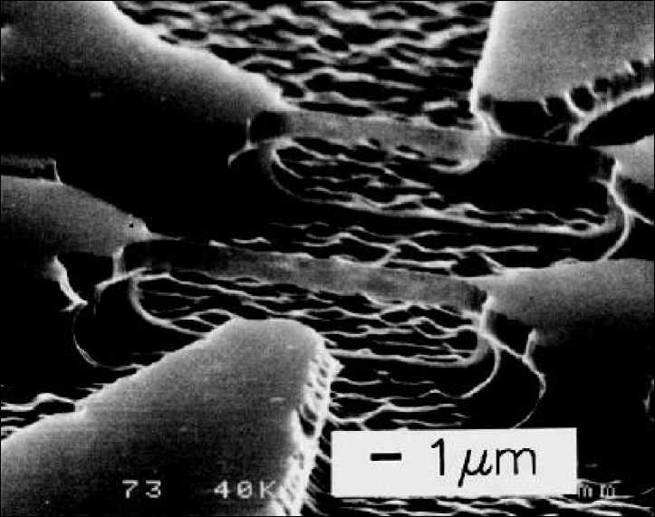
Figure 14. Scanning electron microscope (SEM) micrograph of Si beam
AlN is also piezoelectrically active, with the possible advantage of more straightforward displacement actuation and detection.
The fabrication procedure for a suspended, micron-scale structure involves several steps which we will now outline for the example of a SiN structure; the fabrication procedures for other materials are similar (see, e.g., for a comprehensive review of device fabrication, M. Blencowe, “Quantum electromechanical systems,” Physics Reports, 2004, Vol. 395, No 2, pp. 159 - 222).
The process starts with a single crystal Si (100) wafer on which is grown a few hundred nanometer thick sacrificial layer of silicon dioxide, followed by the deposition of a silicon nitride layer of comparable thickness and finally a bilayer of poly-methylmethacrylate (PMMA) resist (see, Figure 15a).
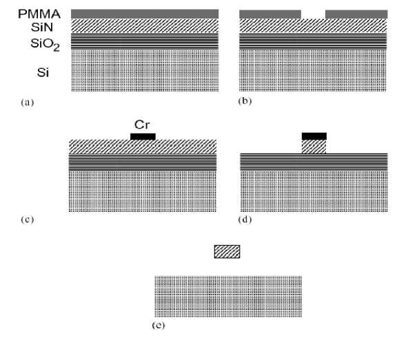
Figure 15. The various steps in the fabrication of a SiN suspended beam structure shown in cross section
The geometry of the suspended structure is then patterned on the resist using electron-beam lithography and the resist developed (see, Figure 15b).
A nice example of a micron scale electromechanical device is the mechanical single electron shuttle shown in Figure 16.
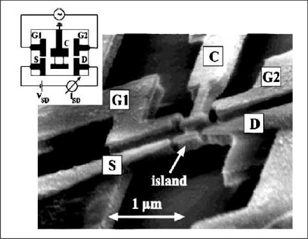
Figure 16. SEM micrograph of micron scale, mechanical single electron shuttle. The cantilever (C) is driven at its fundamental frequency by an ac voltage applied to gates G1 and G2. Electron transport occurs from source (S) to drain (D) via the metallic island at the end of the cantilever
By driving the cantilever close to one of its lowest resonant frequencies, it can shuttle electrons from the source to drain electrode via the small metallic island at the tip of the cantilever. The cantilever resonant frequencies involved are ≤ 100 MHz , while the lowest quoted temperature at which the device is operated is 4.2 K; the cantilever behaves as a classical oscillator.
However, by scaling down the cantilever a bit so as to increase its lowest resonant frequencies and in addition cooling the device down to a few tens of mK, it should be possible to observe in the source–drain I– V characteristics the quantum signatures of single-to-few phonon absorption and emission from these vibrational modes when driven by the shuttling electron current alone (i. e., without the external ac driving of the cantilever).
Remark . By appropriately tuning the SET voltages and capacitance values, it may be possible to achieve the sensitivity at or even better than the quantum zero-point displacement uncertainty limit. However, care must be taken when making sensitivity predictions in the quantum regime which are based on the approximate orthodox model of the SET and classical description of the mechanical resonator. For small displacements of the mechanical resonator, xd , the SET works as a linear amplifier to a good approximation and its quantum dynamics will add an irreducible amount of quantum noise to the input zeropoint signal for phase insensitive detection. While an analysis using the orthodox model suggests that choosing the gate voltage such that the tunneling current is a smaller percentage of the maximum current improves the displacement sensitivity, clearly no meaning can be attached to such sensitivity predictions in small current regions where the quantum noise limit is violated. It is important therefore to go beyond the orthodox model of the SET to include higher order quantum corrections such as co-tunnelling processes. This will enable us to extend the displacement sensitivity analysis to the regime where the incoherent, sequential tunnelling contribution to the current is comparable to or smaller than the co-tunnelling contribution, as well as consider tunnel junction resistance values comparable to or smaller than the quantum of resistance e 2 / й (which may be necessary in order to have measurable currents). Indications from orthodox model analyses suggest that quantum noise-limited detection is possible in this regime. Note that 25
the SET behaves e1ectively as a quantum point contact in the cotunnelling-dominated regime, suggesting that quantum-limited displacement detection may also be possible with a quantum point contact-based displacement detector.
It is essential also that the above noise analysis be extended to describe the fully coupled, quantum dynamics of the combined SET-mechanical resonator system. While the influence of the resonator on the SET and backaction of the SET on the resonator have been partially analyzed, the dynamics loop still needs to be closed whereby the resonator’s motion influences the SET which in turn acts back on the resonator and so on. Some progress has been made, which describes the fully-coupled classical dynamics of SET-resonator system, while it describes the quantum dynamics of a single level quantum dot coupled to a mechanical resonator, viewed as a simplified model of the SET-resonator system. The coupled dynamics becomes especially interesting and non-trivial when the gate voltage is increased beyond the optimum operating point and longer, more floppy resonators are used such that there is a large, fluctuating back action force on the resonator due to the electrons tunneling onto and o1 the SET island. The resulting fluctuating motion of the resonator in turn affects the SET’s tunneling current and can for example be detected as a peak in the current noise about the cantilever’s resonant frequency. By examining the dependence of the peak height and width on the drain–source and gate voltages of the SET, information can be gained about the intrinsic island voltage noise characteristics of the SET at the resonator frequency. This is somewhat analogous to the coupled tunnel junction-mechanical oscillator system analyzed. Also of relevance is a theoretical investigation of the electromechanical noise due to an electron current transferring momentum to a suspended quantum wire through which it flows.
The coupled quantum dynamics of the SET-resonator system first requires the derivation of a master equation for the quantum state density matrix in, say, the SET island number and resonator (oscillator) number basis representation. The master equation can be obtained in a systematic way from the full, microscopic Schrödinger equation using the diagramatic method. A complementary formalism which can also be used to investigate the coupled quantum dynamics is the so-called quantum trajectories approach. This approach will yield a description of the evolution of a single mechanical oscillator undergoing continuous measurement by the SET displacement detector. Averaging over individual SET drain–source current time traces (the measurement records) obtained within the trajectories formalism will give the ensemble-averaged current obtained from the master equation. Similarly, averaging over the position trajectories of the oscillator interacting continuously with the SET and subject to damping and noise from its environment (other than the SET), will give the oscillator’s ensemble-averaged position obtained from the master equation. One application of the trajectories approach is to active feedback control, whereby the information gained about the state of the oscillator through continuous monitoring by the SET is used to control the oscillator’s subsequent evolution so as to cool the oscillator down (for example, see below).
Example : Experimental progress towards quantum-limited SET-based displacement detection . A necessary step towards realizing a rf-SET displacement detector with sensitivity at or below the quantum zero-point limit will be to first demonstrate a rf-SET electrometer operating at the fundamental, charge detection sensitivity limit given by the intrinsic shot noise of the SET tunneling current. In the more traditional, low frequency dc-SETs the equivalent input charge noise is dominated by 1/ f noise due to the random excitations of charge traps located in the tunnel junction dielectric, device substrate, or oxide layer covering the island. At sufficiently high frequencies, shot noise and amplifier noise are expected to dominate over 1/ f noise. A rf-SET is demonstrated in the superconducting state with a charge sensitivity of 3.2 x 10 - 6 e / V Hz for a 2 MHz signal. The shot noise is responsible for about 60% of the total noise, with the remaining percentage due to amplifier noise. It will also be important to investigate whether such charge sensitivities close to the shot noise limit can be maintained as the gate voltage is increased, so that we are working about a higher number current peak. As discussed earlier, this increases the coupling between the SET and gated mechanical resonator.
Having demonstrated a rf-SET electrometer with sensitivities close to the shot noise limit, the next step is to integrate it with a micron-scale, gated mechanical resonator such as a bridge or cantilever. The first experimental realization of a SET-based displacement detector, where the SET operates as a radio-frequency mixer, is described (see, Figure 17).
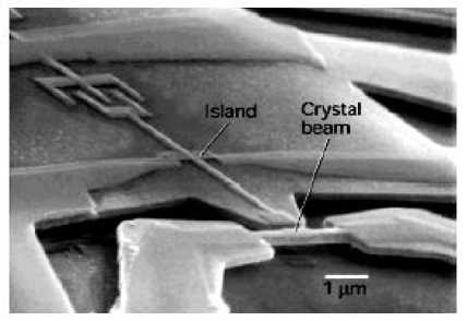
Figure 17: SEM micrograph showing the doubly-clamped GaAs beam and aluminium surface electrodes forming the SET and beam electrode
A sensitivity of 2 x 10 - 5 A / V Hz was demonstrated for a 117 MHz bridge resonator with Q = 1700 at 30 mK. This sensitivity is only about two orders of magnitude larger than the quantum zero-point uncertainty of the resonator. The dominant noise source was the second-stage amplifier; it was estimated that such noise could be reduced by a factor of ten with improved electronics.
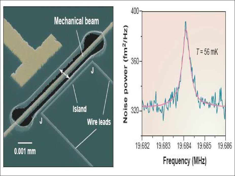
The first demonstration of a displacement detector based on the rf-SET (see, in details Figure 18) achieved a sensitivity of 3.8 x 10 - 5 A / VHz for a 19.7 MHz bridge resonator with Q = 3.5 x 10 4 at 56 mK.
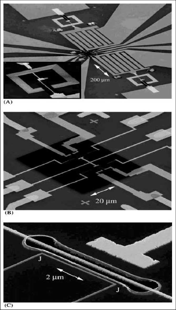
Figure 18: SEM micrograph of the rf-SET displacement detector
This sensitivity is within an order of magnitude from the quantum zero-point uncertainty of the resonator (see, Figure 19).
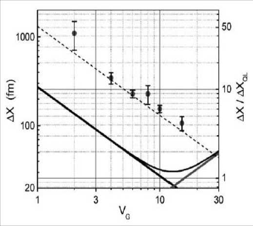
Figure 19: Position sensitivity for the rf-SET displacement detector versus gate voltage
V g
Remark . Note that, while the sensitivities for the two demonstrated displacement detectors are similar, the sensitivity of the device is an order of magnitude closer to the quantum zero-point uncertainty as compared with the other device. This is because the resonator has a lower frequency ν m and higher Q, hence narrower signal bandwidth and larger zero-point uncertainty than the abovementioned resonator. The sensitivity of the rf-SET displacement detector can be improved by increasing the tank circuit quality factor
R to its optimum, matching value Q □ -d . However, as stated earlier, this reduces the detection bandwidth
-
T R 0
and hence the resonator frequency, making it more challenging to cool to the zero-point limit. For the tank circuit, ν = 1.35 GHz and Q ≈ 10 , giving a bandwidth of about 70 MHz. An alternative is to reduce the noise in the second-stage amplifier.
Remark . Figure 18A shows the interdigitated capacitor and square coil inductor (inset) which form a 1.35 GHz LC-resonator. Figure 18B shows a pair of SETs and doubly-clamped beams on the SiN membrane (dark square). Figure 18C is a close-up of a SET and SiN beam with Au electrode. The tunnel junctions are at the corners marked “J”. The Au gate to the right of the resonator controls the SET bias point.
Remark . The solid line is the calculated sensitivity limited by shot noise and backaction noise. The data points are the actual, measured sensitivity, limited by the second-stage, cryogenic microwave amplifier noise.
To achieve better displacement sensitivities, it will also be essential to locate the mechanical resonator closer to the SET island than has been achieved ( 0.25 μm gap) and ( 0.7 μm gap). This is so as to increase the gate capacitance, and hence the coupling strength between the metallized mechanical resonator and SET island. A possible alternative method to achieve strong coupling between the mechanical resonator and SET is to fashion the former out of a piezoelectric material. The SET can then be located directly on resonator’s surface, sensing changes in the polarization charge due to motion-induced strain in the resonator, analogously to the FET strain sensors mentioned earlier. This avoids the problem of having to define a small gap between the resonator and separated SET.
The nano-mechanical resonator is a long thin bridge formed on a layered wafer by etching out the substrate beneath it. The bridge is driven with a magnetic field, and oscillates up and down at 20MHz. On the near side of the resonator is a single electron transistor (SET), whose central island is formed by the two junctions marked “J”. On the far side is a T-Shaped electrode or “gate”. The voltage on this gate is varied and this results in a varying force on the resonator. Image is courtesy of Keith Schwab. Since the oscillator is harmonic, classical LQG theory can be used to obtain an optimal feedback algorithm for minimizing the energy of the resonator, so long as one takes into account the quantum back-action noise caused by the 29
measurement. The details involved in obtaining the optimal feedback algorithm and calculating the optimal measurement strength are given below. It has further been shown that adaptive measurement and feedback can be used to prepare the resonator in a squeezed state.
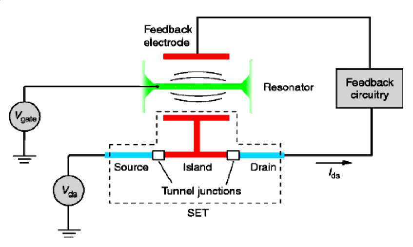
To perform such feedback cooling the resonator must be monitored, and the result feedback in real time to affect the dynamics. A practical method of performing a continuous measurement of the position of the resonator is to use a single-electron transistor (SET). To measure the position of the resonator one locates the central island of the SET next to the resonator. When the resonator is charged, and the SET is biased so that current flows through it, changes in the resonator’s position alter the potential on the central island, which in turn changes the current. The current therefore provides a continuous measurement of the position of the resonator, and this is just what is required for implementing a linear feedback cooling algorithm. A feedback force can be applied by applying a voltage to a gate capacitively coupled to the resonator, and adjusting the voltage so as to damp the resonator (see, Figure 20), or by passing a variable current through the oscillator in the presence of a fixed external magnetic field.
(a)
(b)
Figure 20: A schematic of the resonator (a), measuring, and feedback apparatus (b)
Remark . Electron micrograph of the device in Figure 20a (left) showing the mechanical beam and single-electron transistor wire leads and island. Electrons tunnel one at a time across electrically insulating junctions located at the corners (J). Frequency spectrum (right) of the thermal Brownian motion of the mechanical beam is measured by the single-electron transistor. The temperature of the beam inferred from the spectrum is 56 mK. This is the lowest measured beam temperature achieved in the experiment. The beam displacement units are in femtometers (1 fm = 10 - 5 m).
As the resonator moves closer to the SET, the current flowing through the SET changes, and that information is then used to generate a feedback voltage applied to an actuating gate. We will analyze below the first system, although the results should apply to the second as well. In the analysis we will use the theory of the dc-SET. While an experiment would most likely use a radio-frequency (rf) SET the characteristic frequency of a SET is typically of the order of 10 GHz, so that the rf drive looks constant to the SET, and the dc-SET equations can be used.
The second example of feedback control we consider is that of cooling an atom trapped in an optical cavity (see, for example, Figure 21).
An optical cavity consists of two parallel mirrors with a single laser beam bouncing back and forward between them. The laser beam forms a standing wave between the mirrors, and if the laser frequency is chosen appropriately, a single atom inside the cavity will feel a sinusoidal potential due its interaction with the standing wave. It is therefore possible to trap an atom in one of the wells of this potential. It turns out that information regarding the position of the atom can be obtained by monitoring the phase of the light which leaks out one of the mirrors. Specifically, the phase of the output light tells the observer how far up the side of a potential well the atom is. In addition, by changing the intensity of the laser beam that is driving the cavity, one changes the height of the standing wave, and thus the height of the potential wells. In this system we therefore have a means to monitor the atom and to apply a feedback force.
A feedback algorithm can be used to cool the atom to its ground state. Actually, the algorithm will prepare the atom either in its ground state, or its first excited state, each with a probability of 50%. However, from the measurement record the observer know which one, and can take appropriate action if the resulting state is not the desired one.
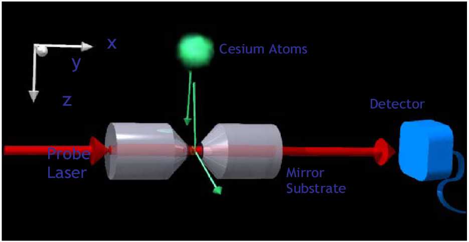
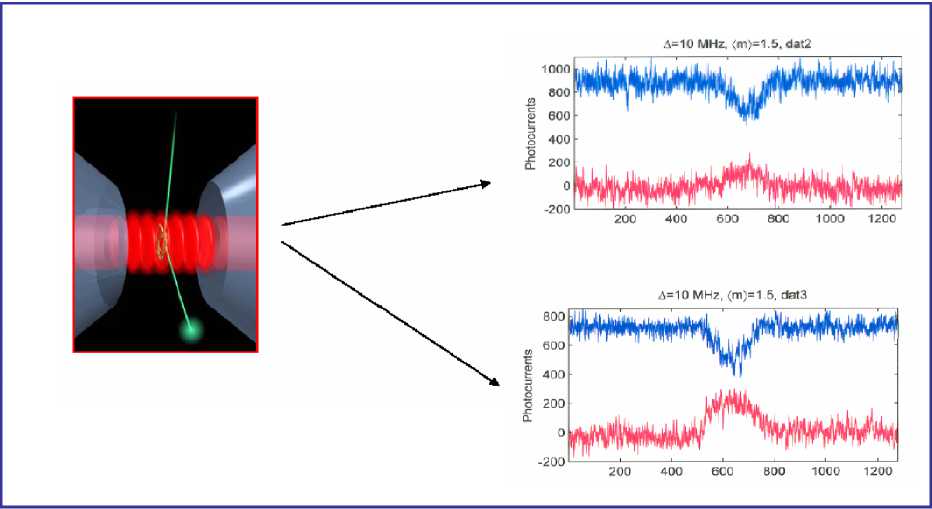
Figure 21: Cavity QED with cold atoms
If the location of the atom was known very accurately, then we could use the following feedback algorithm to reduce its energy: increase the height of the potential when the atom is climbing up the side of a well, and reduce it when the atom is falling down towards the centre. This way the energy of the atom is reduced on each oscillation, and the atom will eventually be stationary at the centre of the well. However, it turns out that this algorithm is not effective, either classically or quantum mechanically, when the variance of atom in phase space is appreciable. The reason is that the cyclic process of raising and lowering the potential, which reduces the energy of the atom’s mean position and momentum, actually increases the variance of the phase-space probability density. Classically we can eliminate this problem by observing the atom with sufficient accuracy, but quantum mechanically Heisenberg’s uncertainty relation prevents us from reducing the variance sufficiently.
As a result, an alternative algorithm is required.
and switch it low when the resulting energy increase is minimal, in a similar fashion to the classical algorithm described above. The result is that the atom will lose motional energy on each cycle. The curious effect whereby the atom will cool to the ground state only half the time is due to the symmetry of the system, and the fact that the feedback algorithm respects this symmetry.
Conclusions
Specifically, the feedback process cannot change the average parity of the initial probability density. Since the ground state has even parity, and the first excited state odd parity, if the initial density of the atom has no particular parity (a reasonable assumption), then to preserve this on average the process must pick even and odd final states equally often. Full details regarding the feedback algorithm and the resulting dynamics of the atom is given.
Although we do not have the space to describe them here, applications of feedback control have been proposed in a variety of other quantum systems. Three of these are cooling the motion of a cavity mirror by modulating the light in the cavity, controlling the motion of quantum-dot qubits, and preparing spin-squeezed states in atomic clouds. In addition, feedback control has now been experimentally demonstrated in a number of quantum systems.
Namely in optics, cold atom clouds, and trapped ions. As example, we will demonstrate a fast, robust and non-destructive protocol for quantum state estimation based on continuous weak measurement in the presence of a controlled dynamical evolution. The experiment uses optically probed atomic spins as a testbed, and successfully reconstructs a range of trial states with fidelities of ~ 90%. The procedure holds promise as a practical diagnostic tool for the study of complex quantum dynamics, the testing of quantum hardware, and as a starting point for new types of quantum feedback control.
References Introduction in quantum optimal control
- A.G. Butkovskii, and Yu.I. Samoilenko, Control of quantum-mechanical processes. - Nauka, Moscow, 1984 (English translation: Kluwer Academic Publishers, Dordrecht, 1990).
- M. Dahleh, A. Pierce, H. Rabitz and V. Ramakrishna, Control of molecular motion // Proc. IEEE, 1996, Vol. 84, No 1, pp. 7 - 15.
- H. Rabitz, Controlling quantum phenomena: why does it appear easy to achieve? // J. of Modern Optics, 2004, Vol. 51, No. 16-18, pp. 2469-2475.
- S.A. Rice and M. Zhao, Optical Control of Molecular Dynamics. - Wiley Intersicence Publication, 2000.
- M. Shapiro and P. Brumer, Principles of the Quantum Control of Molecular Process. - Wiley Intersicence Publication, 2003.
