Investigations of Cellular Automata Linear Rules for Edge Detection

Published Online April 2012 in MECS

Many versions of cellular automata (CA) with three neighborhood local state transition rule are known. In [1], algebraic properties of CA with local state transition rule number 90 are investigated. In [2] and [3], properties of CA’s with cyclic boundary condition are investigated, using a polynomial expression. In [4], properties of CA’s with fixed value boundary condition are investigated, using algebraic integers. These studies mainly deal with three neighbourhood CA’s. But the behaviors of CA’s with five or more neighbors are full of variety [5],[13].

Ulam [6] and Von Neumann [7] at first proposed CA with the intention of achieving models of biological selfreproduction. After a few years, Amoroso and Fredkin and Cooper [8] described a simple replicator established on parity or modulo-two rules. Later on, Stephen Wolfram formed the CA theory [9],[10]. Nowadays, CA are widely used in many tasks because of their useful characteristics and various functions. CA are models for systems which consist of simple components and behavior of each component is obtained and reformed upon the behavior of its neighbors and their previous behavior. The constructing components of these models can do robust and complicated tasks by interacting with each other. Cellular automata are widely used in many areas of image processing such as de-noising, enhancing, smoothing, restoring, and extracting features of images. Detecting the edge components of the image, one of the most important image processing tasks, is used for object background separation, 3-D interpretation of a 2-D image, and pre-processing in image understanding and recognition algorithms [11],[12]. It usually gives as output a binary image in which the edge points have been highlighted. Edge detection is a mandatory step in many image analysis procedures, and the quality of edge detection is a crucial characteristic [13]. Quality is assessed in two different ways: accuracy of edge detection, and level of connectivity in continuous edges. If some edges are still unconnected after edge detection, then an additional edge linking process is required [14],[15].

There are many methods for edge detection, and most of them use the computed gradient magnitude of the pixel value as the measure of edge strength [16]. The early days of works on edge detection are done by Sobel and Roberts [24]. Their detection methods are based on simple intensity gradient operators. Later on, much of the research works have been devoted to the development of detectors with good detection performance as well as good localization performances. A different edge detection method i.e. Prewitt, Laplacian, Roberts and Sobel uses different discrete approximations of the derivative function. For comparison purposes, we have used here four most frequently used edge detection methods namely Sobel edge detection [25], Prewitt edge detection [26], Canny edge detection [28] and Roberts edge detection [27].

A method for the evolutionary design of CA rules for edge detection was proposed by Batouche et al. [17],[ 20]. Khan et. al. studied the nine neighborhood 2DCA [21]. He developed the basic mathematical model to study all the nearest neighborhood 2D CA and presented a general framework for state transformation. P. P. Choudary et al has proposed modeling techniques for fundamental image processing, where they had applied the rules only on binary images [18]. Two dimensional binary CA are used for binary-image edge detection, and transition rule evolution is guided by a genetic algorithm. Another application of this method was done by Rosin and the method was extended to handle gray-scale images [19]. The images are decomposed into a number of binary images with all possible thresholds. Each of the binary images is processed using binary CA rules. Nayak used color graphs to model 2D CA linear rules [22]. After that Munshi et. alhas proposed an analytical frame work to study a restricted class of 2D CA [23]. Rosin later applied an improved version of this method to edge detection [20]. However, this method has a very long calculation time due to the iterative process used for hundreds of binary images.

In this paper we have investigate cellular automata linear rules for edge detection and based on this investigation we have classified the rules into no edge detection rules, strong edge detection rules and weak edge detection rules. The idea is simple but effective technique for edge detection that greatly improves the performances of complicated images. The comparative analysis of various image edge detection methods is presented and shown that CA based algorithm performs better than all these operators under almost all scenarios. The paper is organized as follows: CA is defined in section 2. Section 3 begins with a brief description of CA Linear rules, Section 4 shows the classification of the rules and then goes on to the comparative analysis with traditional edge detectors.

• II.    CELLULAR AUTOMATA

CA model is composed of cell, state set of cell, neighbourhood and local rule. Time advances in discrete steps and the rules of the universe are expressed by a single receipt through which, at each step computes its new state from that of its close neighbours. Thus the rules of the system are local and uniform. There are onedimensional, two-dimensional and three-dimensional CA models. For example, a simple two-state, one dimensional CA consists of a line of cells, each of which can take value ‘0’ or ‘1’. Using a local rule (usually deterministic), the value of the cells are updated synchronously in discrete time steps. With a k-state CA model each cell can take any of the integer values between 0and k-1. In general, the rule controls the evolution of the CA model.

A CA is a 4-tuple {L, S, N, F}: where L is the regular lattice of cells, S is the finite state of cells, N is the finite set of neighbors indicating the position of one cell related to another cells on the lattice N, and F is the function which assigns a new state to a cell where F:S|N| S.

As the image is a two dimensional, here we use 2DCA model. In a 2DCA the cells are arranged in a two dimensional grid with connections among the neighboring cells, as shown in the figure (1) and in figire (2). Figure (1) shows the connections of one cell with moore neighborhood whereas as figure (2) shows the grid connection. The central box represents the current cell (that is, the cell being considered) and all other boxes represent the eight nearest neighbours of that cell. The structure of the neighbours mainly includes Von Neumann neighbourhood and moore neighbourhood are shown in figure–(3):

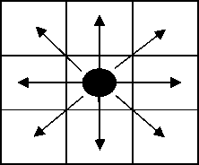
Figure (1): 2DCA transition dynamics

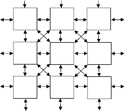
Figure (2): Network Structure of 2DCA

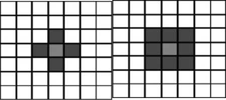
Figure (3) : structure of neighbourhoods

• (a)    Von Neumann neighbourhood

• (b)    Moore neighbourhood

Von Neumann neighbourhood, four cells, the cell above and below, right and left from each cell is called von Neumann neighbourhood of this cell. The radius of this definition is 1, as only the next layer is considered. The total number of neighbourhood cells including itself is five as shown in the equation (1)[10]:

N(I,j) = { (k,l) Є L : |k-i| + |l-j| ≤ 1 }       (1)

where, k is the number of states for the cell and l is the space of image pixels. Besides the four cells of von Neumann neighbourhood, moore neighbourhood also includes the four next nearest cells along the diagonal. In this case, the radius r=1 too. The total number of neighbour cells including itself is nine all as shown in the equation (2)[10]:

N(I,j) = { (k,l) Є L : max (|k-i|,|l-j|) ≤ 1 }         (2)

The state of the target cell at time t+1 depends on the states of itself and the cells in the moore neighbourhood at time t, that is:

S i,j (t+1) = f ( S i-1,j-1 (t) , S i+1,j (t) , S i-1,j+1 (t) , S i,j-1, S i,j (t) , S i,j+1 (t) , S i+1j-1 (t) , S i+1,j (t) , S i+1,j+1 (t) )    (3)

• III.    LINEAR CA RULES

A rule is the “program” that governs the behavior of the system. All cells apply the rule over and over, and it is the recursive application of the rule that leads to the remarkable behavior exhibited by many CA’s. In 2-D Nine Neighborhood CA the next state of a particular cell is affected by the current state of itself and eight cells in its nearest neighborhood also referred as Moore neighborhood as shown in Figure (1).

16	8	4
32	1	2
64	128	256

Figure (4): 2DCA Rule Convention using moore neighborhood

Therefore, 2⁹ = 512 possible states exist. Each of 512 states can produce a 1 or a 0 for the centre cell in the next generation. Hence, 2⁵¹² possible rules exist. A comprehensive study of all rules in higher dimensional automata is thus not easily possible. However, in this paper we will mainly concentrate on the 512 linear rules. i.e. the rules, which can be realized by EX-OR operation only. A specific rule convention that is adopted here is given by [21].We use their model as reference and modify it so as to study CA based image processing.

The central box represents the current cell and all other boxes represent the eight nearest neighbours of that cell. The number, within each box represents the rule number associated with that particular neighbour of the current cell. In case, the next state of a cell depends on the present state of itself and/or its one or more neighbouring cells (including itself), the rule number will be the arithmetic sum of the numbers of the relevant cell.

• IV.    methodologies

The methodology that we take is shown in the figure (5). These steps are explained as follows:

Step 1: First of all, it is necessary to read the data information that composes the image. It does not matter the format of the image (e.g. jpeg, bmp, png, gif, etc), we assume that all image data is formed by a data matrix of size M x N.

Step 3: We set up the cellular automata map which where the edge detector operation will be performed. This can be directly done by separating each pixel of the original image into one cell. As the image information is composed of a data matrix of size M x N, the cellular automata map will be also in the shape of a M x N matrix, thus with MN cells.

Step 4: Once we have a cellular map of the monochrome image data, we then add null-boundary condition to the cellular automata map in order to avoid the boundary conditions. Remembering that in this project the adopted model is the Moore Neighborhood Model.

Step 5: We apply an edge detection rule in order to select the characteristics of processing of the image. A detailed explanation of the “edge detection rules” is to be made in the next section.

Step 6: The final result is a monochrome edge detected image. The pixel size (number of columns and rows of the image data matrix) will be exactly the same as that of the original image data.

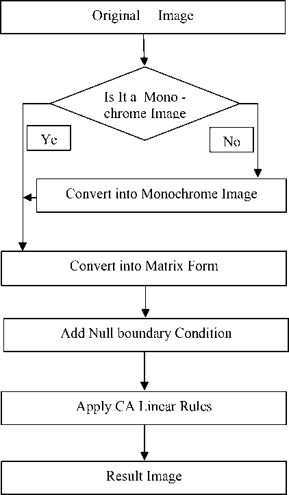
Figure (5): Proposed Methodology

• IV.    Experimental results

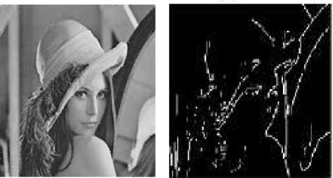
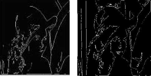
The experimental image is selected as the classical Lena image, whose sizes is 256×256 as shown in figure (1) . Here, we apply all 512 CA linear rules to the classical Lena image and found the following three results as shown in figure (6).

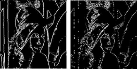
(c)                            (d)

Figure (6): Results on Lena Image

Quality is assessed in two different ways: accuracy of edge detection, and level of connectivity in continuous edges. Here, we classify all the 512 CA linear rules into three groups based on the patterns of edge detection that is the rules showing no edge detection, rules showing strong edge detection and rules showing weak edge detection. These three groups are shown in figure (4), figure (5) and figure (6). Group 1 rules shows the pattern of figure (6.b), group 2 rules shows the pattern of figure (6.c) whereas group 3 rules shows the patterns of figure (6.d) .

Figure (7) shows the comparative results of the proposed method and the traditional methods of edge detection, whereas figure (7.a) is the original image, figure (7.b) is the image obtained after applying the proposed model, figure (7.c) is the edged image produced by the Sable method and figure (7.d) is the edged image produced by Canny method. It is clearly visible from the results that the proposed method is the best method than the traditional methods of edge detections.

(c)                              (d)

Figure (7): Comparative results on Lena Image.

1,2,4,7,8,11,13,14,16,19,21,22,25,26,28,31,32,35,37,38,41,42, 44,47,49,50,52, 55,56,59,61,62,64,67,69,70,73,74,76, 79,81, 82,84,87,88,91,93,94,97,98,100,103,104,107,109,110,112,115, 117,118,121,122,124,127,128,131,133,134,137,138,140,143, 145,146,148,151,152,155,157,158,161,162,164,167,168,171, 173,174,176,179,181,182,185,186,188,191,193,194,196,199, 200,203,205,206,208,211,213,214,217,218,220,223,224,227, 229,230,233,234,236,239,241,242,244,247,248,251,253,254, 256,259,261,262,265,266,268,271,273,274,276,279,280,283, 285,286,289,290,292,295,296,299,300,301,302,304,307,309, 310,313,314,316,319,321,322,324,327,328,331,333,334,336, 339,341,342,345,346,348,351,352,355,357,358,361,362,364, 367,369,370,372,375,376,379,381,382,385,386,388,391,392, 395,397,398,400,403,405,406,409,410,412,415,416,419,421, 422,425,426,428,431,433,434,436,439,440,443,445,446,448, 451,453,454,457,458,460,463,465,466,468,471,472,475,477, 478,481,482,484,487,488,491,493,494,496,499,501,502,505, 506,508,511.

Figure (2): Group 1, Rules Showing No Edge Detection

3,5,10,12,17,18,20,23,24,27,29,30,33,34,36,39,40,43,45,46, 51,53,58,60,65,66,68,71,72,75,77,78,83,85,90,92,99,101,106, 108,113,114,116,119,120,123,125,126,130,132,139,141,144, 147,149,150,153,154,156,159,160,163,165,166,169,170,172, 175,178,180,187,189,192,195,197,198,201,202,204,207,210, 212,219,221,226,228,235,237,240,243,245,246,249,250,252, 255,257,260,263,264,270,272,275,277,278,281,282,284,287, 288,291,293,294,297,298,300,303,305,311,312,318,320,323, 325,326,329,330,332,335,337,343,344,350,353,359,360,366, 368,371,373,374,377,378,380,383,384,390,393,399,400,402, 404,407,408,411,413,414,417,418,420,423,424,427,429,430, 432,438,441,447,449,450,452,455,456,459,461,462,464,470, 473,479,480,486,489,495,497,498,500,503,504,507,509,510

Figure (3): Group 2, Rules Showing Strong Edge etection

6,9,15,48,54,57,63,80,86,89,95,96,102,105,111,129,135,136, 142,177,183,184,190,209,215,216,222,225,231,232,238,258, 267,269,306,308,315,317,338,340,347,349,354,356,363,365, 387,389,394,396,435,437,442,444,467,469,474,476,483,485, 490,492.

Figure (4): Group 3, Rules Showing weak Edge etection

• V.   Conclusions

In this paper we have investigated CA linear rules for edge detection. We have tested all the rules and based on the investigation we have classified the rules into three groups, rules shows no edge detection, rules showing strong edge detection and rules showing weak edge detection. By experimental comparison of different methods of edge detection we observe that the proposed method leads to a better performance. The experimental results also demonstrated that it works satisfactorily for different digital images. This method has potential future in the field of digital image processing. The work is under further progress to examine the performance of the proposed edge detector with noise filtering for different digital images affected with different kinds of noise.