Irregular Function Estimation with LR-MKR

Published Online February 2011 in MECS

Learning to fit irregular data with noise is an important research problem in many real-world data mining applications, which can be viewed as a function approximation from sample data. Kernel tricks have attracted more and more research attention recently. For kernel methods, the data representation should be implicitly chosen through the kernel function. Because this kernel actually plays several roles: it defines the similarity between two examples X and X ' , while defining an appropriate regularization term for learning problem. Choosing a kernel K is equivalent to specifying a prior information on a Reproducing Kernel Hilbert Space (RKHS), therefore having a large choice of RKHS should be fruitful for the approximation accuracy, if over fitting is properly controlled, since one can dapt its hypothesis space to each specific data set [1]-[3]

For given data set S = {( X i , y _; )} " = 1 . Assume that m ( X ) G H , where H is some reproducing kernel Hilbert space called active space, with respect to the reproducing kernel K . The square norm related to the inner product by || f || H = ^ f , f^ H . Consider the problem,

n min H (m ) = ^ L (yi, m (xi)) + XP (m )

i = 1

Where X is a positive number which balances the tradeoff between fitness and smoothness; L is a loss function which determines how different between y_i and m ( x_i ) and should be penalized; P ( m ) is a function which denotes the prior information on the function m ( • ) . When the penalized function P ( • ) is defined as p ( m ) = || m || H . By the represent theory, the solution of the upper kernel learning problem is of the general form n

^{m ( x} ) = ^ « ^{К ( x} , x i )               ⁽¹⁾

i = 1

Where ai are the coefficients to be learned from the examples, while K is positive definite kernel associated with RKHS H . It should be noted that m can also be expressed with regards to the basis elements of H as

m(X) = ^aiфi(X) , which is called the dual from of m . An advantage of using the kernel representation given in (1) is that the number of coefficients to be estimated depends only on n and not on cardinality of the basis, which may be infinite. It is this properly that makes the kernel methods so popular, see, e.g. [16].

Recently, using multiple kernels instead of a single one can enhance the interpretability and improve performance [1]. In such cases, a convenient approach is to consider:

NN

K ( x , x ') = £ C i K i ( x , x '), 5,t . ^ C i = 1, C i >  0     (2)

i = 1                               i = 1

Where N is the total number of kernels. Interpretability can then be enhanced by a careful choice of the kernels, K j and their weighting coefficients, ci . Each basis kernel K j may either use the full set of variables describing x or only a subset of these variables. Within this framework, the multiple kernel learning problem is transformed to learning both the coefficients ai and the weights cj in a single optimization problem. Unfortunately, it is difficult problem to search the optimal parameters in 2-dimention space in irregular function regression problem. In addition, it ignored that a sequence of kernels will induce representation redundancy inevitably and will increase computational burden as a result of much more parameters. Also, the correct number of kernels N is unknown, and simultaneously determining the required number of kernels as well as estimating the associated parameters of MKL is a challenging problem [1].

For irregular functions which comprise both the steep variations and the smooth variations, it is sometimes unsuitable to use one kernel even if a composite multiple kernel with several global bandwidths to estimate the unknown function [2]. First, the kernels are chosen prior to learning, which may be not adaptive to the characteristics of the function so that under fittings and over fittings occur frequently in the estimated function [3]. Although, the localized multiple kernel learning proposed in [4] is adaptive to portions of high and low curvature, it is sensitive to initial parameters. Second, how to determine the number of kernels is unanswered. Finally, classical kernel regression methods exhibit a poor boundary performance [5][6][7]. In order to estimate an irregular function, this paper proposed an improved Nadaraya-Watson estimator approach to produce localized data-driven reweighted multiple kernel learning method; Different from classical MKL, we solve the MKL problem in a series decreased active subspace. Simulations show that the performance of the proposed method is systematically better than a fixed RBF kernel.

The rest of this correspondence is organized as follows. In section 2, we proposed an iterative localized regression to deal with non-flat function regression problem. Section 3 presented regression results on numerical experiments on synthesis and real-world data sets while section 4 concludes the paper and contains remarks and other issues about future work.

• II.    T HE LOCALIZED REWEIGHTED MULTIPLE KERNEL REGRESSION METHOD

In order to achieve the objects refer to abstract, we suggest adherence to the following recommendations. Different from the simple combination of several basis kernels, we proceed a new multiple kernel learning on a sequence of nested subspaces based on iteration approach. During iteration, the active subspace is decreasing while the classical multiple kernel regression is not.

• A.    The Improved Nadaraya-Watson Estimator

  Nadaraya(1964) [8] and Watson(1964) [9] proposed to estimate m ( x ) using a kernel as a weighting function.

Given the sample data set S = {( x i , y _t )} ” _{= 1}:

• < x ; S )   ^E = 1 K h, ⁽ X ^, x ) y = £ w ( x ; S ) y

E i = ₁ ^K h ^{( x} , x - )      - = 1

n

Where wi (X; S) = [£ Kh (x, x-)]-1 Kh (x, x ) is the i=1

Nadaraya-Watson weights, such that

n

E wj (x; S) = 1, V x j=1

And K h ( x ) = h ^{- 1} K ( x / h ) is a kernel with bandwidth h .

Associating blockwise technique, we propose an improved localized kernel regression estimator which achieves automatic data-driven bandwidth selection [10]. Suppose the initial data set S is partitioned into p blocks denote by SS ₁ , SS ₂ ,..., SS_p with length

p d1,d2,...,dp such that Ebj = n [11]. For given x , if j=1

there is some block SSx such that min{ xi | xi e SSx} < x < max{ xi | xi e SSx} Then the block wised Nadaraya-Watson estimator is given as follows

E x e SS x K h ^{( x} ’ x - ) y

m ( x ; SS_x ) =

E._e® K h ^{( x} , x i ) x e SS x

= E w ( x ; SS ) y -x - e SS_x

As thus, the localized estimator presents the unknown function m without a complicated parameters selection procedure.

• B.    The new regress on method

Given a dataset, S = {(xi, yi), xi e Rn, yi e R} . Assume that m(x) e H, where H is some reproducing kernel Hilbert space called active space, with respect to the reproducing kernel K . The square norm related to the inner product by IIfIIH =(f, Ah ■ Consider the problem, min H (m) = ^^L (yi, m (xi)) + XP (m)      (3)

= 1

Where X is a positive number which balances the tradeoff between fitness and smoothness; L is a loss function; P ( m ) = || m||_H is penalized function. By the represent theory, the solution of equation (3) is [12],

T m ( x ) = ^E a - K ( x , x - )            (4)

= 1

A generalized framework of kernel is defined as

N

K ( x , x ') = E cK i ■( x , x ')         (5)

= 1

Where K i ., i = 1,..., N are N positive definite kernels on the same input space X , and each of them being associated to a RKHS H whose elements will be denoted f and endowed with an inner product ^-, -^., and { c } ^N _{= 1} are coefficients to be learned under the nonnegative and unity constraints

N

E C = 1, C > 0,1 < - < N (6) i = 1

How to determine N is an unanswered problem. For any c t > 0 , Hi is the Hilbert space derived from Hi as follows:

H = {/I/e H,: ^H. <„}

ci

Endowed with the inner product

• (/ , g)H = -1 ( / , g\ c_i

Within this framework, Hi is a RKHS with kernel K ‘ = CiK,. (x, x ) , since m (x) = (m OX K,(x, *)) Hi = (m CX ctK t(x, •)) Hi

Then, we define H as the direct sum of the

RKHS H i . Substituting (5) into (4), an updated equation of (2) is obtained as follows, n

m ( X ) = E a K ( x , x , ) t = 1

nN

= E a E c j KA^x , x )

, = 1       j = 1

Nn

=E cE atKj( x, x)

j = 1       = 1

N

= E m j ^{( x} )

j = 1

Instead of the equation (3), we convert to consider the models for j = 1,..., N ,

n min Hj (mj ) = E L (y, mj (xt)) + j(mj )    (8)

t = 1

Then, the kernel learning problem can thus be envisioned as learning a predictor belonging to a series of adaptive hypothesis space endowed with a kernel function. The forthcoming part explains how we solve this problem.

Assume that a kernel function K1 (•, •) and corresponding reproducing kernel Hilbert space H1 are included, and then we get the initial estimator,

E iE_ ® Kh (x, x) y i m (x) =    j=1   xESSj

1 p

E j = 1 E X, e SS ^K h ⁽ x , x t ) j

The residual function can be obtained, res 1 ( x ) = m ( x ) - m 1 ( x ) e V 1 = H - H ₁ '

If we have introduced t kernels {Kj} j=1, then the estimator can be updated as t        tn

^{m (} x ) = E ^m j ⁽ x ) = EE ^a t ^K j ⁽ x , x , ) j = 1                 j = 1 t = 1

And the residual function, rest (x) = m (x) - zm( x)              (11)

If the measurements of res_t fulfilled certain thresholding criteria, here we employ 2-norm, N = t represents the number of introduced kernels and puts an end to iteration procedure. If not, considering the problem in the decreased subspace H_{t + 1} , compute res _t = y_t — ml(x _t ) and update the sample set

S = {( x_t , res _t )} which can be treated as the limited of the initial data set in H t _{+ 1}. Employing iteration, we will consider a new regression problem on the updated sample data set in a decreased subspace.

Compared with the general multiple kernel learning (MKL), the first advantage is that it needs not to select weights a _t which will reduce much more computation burden and just need to select one kernel bandwidth at each iteration step. Furthermore, the new method is adaptive to the local curvature variation and improves the boundary performance as a result of the introduction of blockwised Nadaraya-Watson estimate technique. At last, the number of kernels introduced will change according to real data settings based on iteration which will avoid under fitting and over fitting problem effectively.

C .LR-MKR Algor thm

The complete algorithm of Iterative Localized Multiple Kernel Reweighted Regression can be briefly described by the following steps:

• 1)    Input S , the max mum terar on step M , the threshold 8 , and N = 1 ;

• 2)    InitiaUza the pHot estimator rh(x ) = 0 , and pHot resdlual e = y ;

• 3)    Update the data set S = {( x j , e j )} " = 1 ;

• 4)    Select kernel K , compute the est mator m ˆ( x ; S ) w th equat on (9);

• 5)    Update the estimator m ( x ) = m ( x ) + ml (x ; S ) ;

• 6)    Update the residuals e = y — m ( x ) , and update N = N + 1 ;

• 7)    Calculate the norm of res dual e .

Repeating the steps from 3) to 7), this process is continued until the norm of residual e is smaller than the pre-determined value 8 or the number of iteration step N is larger than the pre-determined value M .

The algorithm of Localized Reweighted Multiple Kernel Regression algorithm is adaptive to different portions with different curvatures and is not sensitive to noise level and the pilot estimation. One kernel in one interation step the new method avoids the representation redundance problem effectively. Although the choice of optimal kernel and associated parameters have been investigated by many model selection problems, the model parameters are generally domain-specific. The Gaussian kernel is most popularly used when there is no prior knowledge regarding the data.

In order to select parameters, we choose 10-fold crossvalidation: randomly divide the given data into ten blocks and consider the Generalized Cross Validation function is

given as

GCV ( θ ) =

1       _{( m ˆ}( - j )

10 ^∑ j

- m )²

Where θ represents the set of relevant parameters, and m ˆ ^{( - j )} is the estimator of m without the jth block samples of S . Smaller values of the GCV function imply better prediction performance. Thus, among a possible set of parameters, the optimal value is the minimized of the GCV function.

widely used in regression tasks. In the experiment, we generated several versions of data sets with different noise level. Then, we repeated each experiment up to 50 runs and summarized average results in Table 1. From the experimental results, several observations can be drawn. First, compared with single kernel regression, the iterative localized reweighted multiple kernel regression could adapt to different portions with different curvature and it could avoid under fitting and over fitting simultaneously. Second, the proposed method shows a better boundary performance. At last, the numerical results show that the new method is less sensitive to the

Ш . EXPERIMENT RESULTS

We have conducted studies on simulated data and real-world data using the proposed method. Each experiment is repeated 50 times with different random splits in order to estimate the numerical performance values. Some of the results are reported in the following. We decide to use, as it is done often, Gaussian radial basis kernel which not only satisfies Mercer’s conditions for kernels, but also is most widely used. Mercer’s conditions are illustrated in Scholkopf (2002) [3]. In classical MKL, it rises not only how many kernels to chose but also which one to choose.

• A.    Application to Simulated Data (1)

At first, we consider the test function

m ( x ) = 5sin(2 x ) exp( - 16 x ² /50)

To examine the performance of regression algorithm. In this experiment, three random samples of size 100, 200, 500 were generated uniformly from the interval [-5,5], respectively. The target values are then corrupted by some noise with a normal distribution N (0, σ ²) . The standard deviation σ is 0.4 and 1, which determines the noise level.

Which has different curvature for different design, so a global bandwidth can not deal with well. It is well known that around the peak of the true regression function m ( x ) the bias of the estimate is particularly important. So, in such areas, it would be better to choose a small bandwidth to reduce these bias effects. Conversely, a larger bandwidth could be used to reduce variance effects, without letting the bias increase too much, when the curve is relatively flat [14]. Experiments result shows that the new method could deal this intrinsic shortcoming well combining with the improved Nadaraya-Watson estimation and iteration approach.

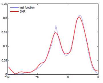
Figure 1 presents the curves of the test function (slender line) and the estimation curves (bold line) when the additive Gaussion noise is N (0,1) . Figure 1(a) demonstrates the test function and sample data; Figure 1(b) shows the estimated curve using the proposed method with two step iteration which deals well with different portions with different curvature; Figure 1(c) demonstrates the standard single kernel regression based on Gaussian kernel with a global bandwidth which was determined through GCV. The mean-square error (MSE) is adopted as the performance metric, which has been noise level when the sample size is fixed.

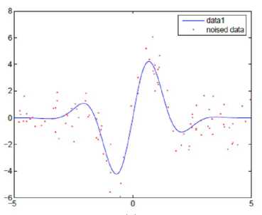
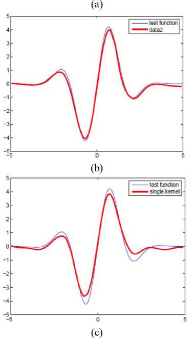
Figure 1. Demonstration of LR-MKL results: the test function (slender line) and the approximation function (bold line). Figure (a) demonstrates the test function and noised sample data; Figure (b) shows the estimated curve using the proposed method which deals with well with different portion of different curvature; Figure (c) demonstrates the standard single kernel regression results( σ = 1 ).

TABLE I. THE AVERAGED EXPERIMENTAL RESULTS OVER 50 REPETITIONS FOR EACH SITUATION . AND THE MSE IS ADOPTED AS THE METRIC

	n
	100	200	500
с = 0.4	0.0226	0.0152	0.0074
C = 1	0.0258	0.0157	0.0076

(a)

(b)

(c)

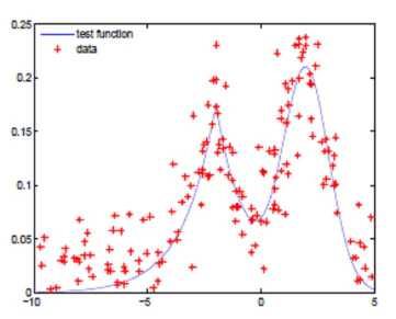
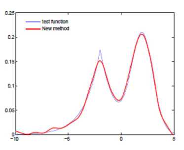
Figure 2. The test function (slender line) and the approximation function (bold line). Figure (a) shows simulated data with white noise (SNR=20); Figure (b) shows the estimated curve using the new method; Figure (c) demonstrates the standard single kernel regression result.

• B.    Application to Simulated Data (2)

The test function is the mixture of Gaussian and Laplacian distributions define by

1        - ( x - 2) 2

m ( x ) = —^— e  ²

2V2n

₊ ⁰⁷ _e -°'⁷I x ⁺²I

The number of data points for experiment is 200, and the experiment was repeated 50 times. Figure 2(a) shows the target values which were corrupted by white noise. The performance of the experiment was shown in Figure 2, in which the slender line present the true test function and the bold line represented the estimated results. Figure 2(b) represented the estimated curve using the proposed method with two step iteration which deals well with different portions with different curvature; Figure 2(c) demonstrated the standard single kernel regression based on Gaussian kernel with a global bandwidth. For this example, it can be seen that the Iterative Localized Multiple Kernel regression method achieved the better performance. Compared with the proposed method, the single kernel regression could not avoid under fitting and over fitting simultaneously and sensitive to the noise at boundary area.

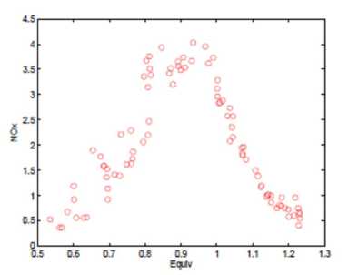
• C.    Application to real data: Burning Ethanol Data

  In order to evaluate the performance of our proposed method in practice, we analyzed the Burning Ethanol Data set. Figure 3(a) shows the data set of Brinkmann (1981) that has been analyzed extensively. The data consist of 88 a measurement from an experiment in which ethanol was burned in a single cylinder automobile test engine. Because of the nature of the experiment, the observations are not available at equally-spaced design points, and the variability is larger for low equivalence ratio.

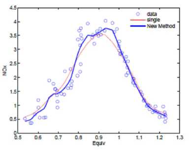
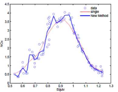
As we all know, it is a difficult problem to control the pump around 0.8. Figure 3 shows the Iterative Localized Multiple Kernel regression results with different parameters and iteration steps. The red line represents the single kernel estimator. The blue in figure 3(b)-(c) represent the estimators after two and three steps iteration with different kernel bandwidths which are determined by GCV. From the experimental results, several advantages can be drawn. First, all the estimated curves have not a spurious high-frequency feature when the equivalence ratio is around 0.8 which is the drawback other regression methods must deal with cautiously. Second, compared with [13], the proposed method is not sensitive to the pilot estimator and the kernel bandwidth selection. Finally, all the fitting results show the good boundary performance.

• D.    CUP Time

All the experiments were implemented in the environment of MATLAB-7.0 on 2.6 GHz Pentium 4 machine with 2-G RAM. Table 2 presents the average CPU time (second) of the general single kernel regression (SK) and the proposed method (LR-MKR) on simulation 1 for three training sample sizes 100, 200, 500, each sample size has been run 50 times. It can be seen that the proposed method needs more CPU time than the general single kernel regression as a result of multiple kernels to be introduced.

(a)

(b)

(c)

Figure 3. Figure (a) shows Burning Ethanol Data; The blue bold lines in figure (b) and (c) show different estimated curves with two and three kernels.

TABLE II.      TRAINING TIMES ( SECONDS ) OF GENERAL SINGLE

KERNEL REGRESSION ( SK ) AND THE NEW METHOD ( LR - MKR ) ON SIMULATION 1.

Sample size	100	200
100	0.3120	0.3276
200	0.3588	0.9204
500	2.7456	5.5068

IV. CONCLUSIONS AND DISCUSSION

In this paper, we consider the kernel trick and proposed an iterative localized reweighted multiple kernel regression method which includes two parts. At first, an improved Nadaraya-Watson estimator is introduced based on blockwised approach to produce an localized data-driven reweighting method, which improves the classical Nadaraya-Watson estimator to be adaptive to different portions with different curvatures; Then, considering the shortcoming of general multiple kernel regression, we convert to iteration in a series decreased active subspaces and proposed a novel kernel selection framework during iteration procedure which simultaneously avoids under fitting and over fitting effectively. The presentation covers the curves both deep variation and smooth variation. The simulation results show that the proposed method is less sensitive to noise level and pilot selection. Furthermore, experiments on simulated and real data set demonstrate that the new method is adaptive to the local curvature variation and could improve boundary performance effectively. It is easy to extend the method to other type additive noise. Kernel function plays an important role in kernel trick and can only work well in some circumstances, so, how to construct a new kernel function according to the given sample data settings is another direction we will keep up with.