Island Loss for Improving the Classification of Facial Attributes with Transfer Learning on Deep Convolutional Neural Network

The human face can provide lots of information like his age or emotional state. So, the understanding facial feature is an important task in machine intelligence. Much of these tasks can be treated as a classification task but classification on facial feature is harder than other classification in most cases. This is because there is a lot of similarities in different classes of this kind of classification task. For example, different people have different ways of expressing the same emotion and the difference between some emotions are very little. Similarly, people of different geographic area or lifestyle has a different aging effect on the face of the same age.

Expression of emotion is important in social communication. Human expresses emotion through facial expression, speech, and body movement. Emotion recognition has many commercial uses at consumer level products such as understanding users’ satisfaction for movie or service. Many other real-world applications will be benefited from this application like effect-aware game development and call center. This is a challenging problem because of the very nature of the human face. The main reason for this complexity includes the overlapping of facial expression in different people and different people have a different way of expressing emotions.

Emotion recognition is extensively studied due to its numerous practical application. From classical feature detection to recent deep learning techniques. Any type of audio-visual signal, e.g. image, video, text, speech, and biosignals can be used as input to the emotion detection system. However, vision is the most important and most meaningful source of information for understanding human emotion. In the case of vision-based emotion recognition system factors like the human facial pose, context and action provide valuable insight. Most of the datasets [1,2,3,4,5,6,7,8] for human facial emotion recognition system is collected in lab condition where the subjects are told to create artificial emotional which is far from natural. So, when it comes to the fact of understanding emotion in a real-life situation, the task becomes very difficult and the accuracy drops drastically. Understanding emotion in an uncontrolled environment still remains a challenge for researchers due to facts such as low-resolution occlusion, culture and age difference.

The facial emotion recognition task can be divided into two categories depending on the source: static image and video sequences. For sequence-based strategies, the sequence of frames with other object and events can provide useful strategies for finding facial highlights. Nonetheless, facial emotion detection from a static image is more challenging than that of video as there is no extra information available. However, in sequence-based models, a natural face is used as a baseline. Which has to be determined first. At that point, the recognition is based on the baseline face. Therefore, the determination of the baseline image is very important. If the baseline face is not determined properly, the recognition will not be accurate.

Among the earlier successful methods, appearancebased approaches were very popular. These methods are based on the linear discriminant analysis (LDA) which finds patterns in data. But these encounters difficulties

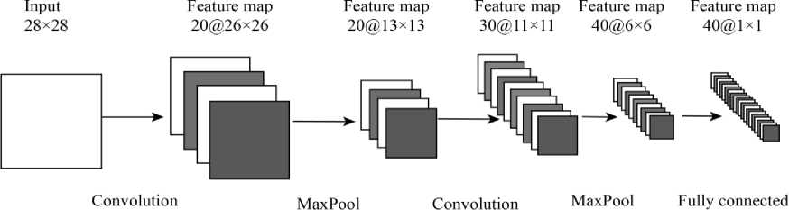
Fig. 1. The architecture of a Convolutional Neural Network. The example shows the processing of a 28 × 28 size image. It takes an image as input and apply convolution and MaxPolling of the image and finally convert it into one dimensional vector.

ImageNet Dataset

Task specific data (facial emotion dataset)

Training

Fine Tuning

Deep Neural Network

Pretraind State

Trained model

(on ImageNet)

Fig. 2. Steps of training using the Transfer method. First the model is pre-trained with standard laege dataset to get the pre-trained stage. This is then fine-tuned on task specific data.

with high dimensional data. Several methods have been proposed to solve the high dimensional issues. A novel regularized method was proposed in [9] to solve the high dimensional problem. Also, fuzzy logic was introduced to recognize facial expression [10].

Some other approaches include Hidden Markov model and the Bayesian network. Such detection starts with face detection algorithm [11] which is followed by feature extraction algorithms [12,13,14]. This output vector gives features vector which is processed by classifier algorithms to generate output. Although these models were successful in many application including classification, it did not do very well because of two reasons associated with emotions recognition. First, understanding emotion requires a moderately high-resolution image which means working with high dimension data. Second, the difference in faces among different emotion state is very low which makes the classification task harder. Another popular technique in machine learning is ensemble learning. Kim et al. [15] used an ensemble-based method with varying based architecture and parameters that gave an accuracy of 61% in EmotiW2015.

Age estimation is another interesting and challenging literature nowadays. A good number of methods have been studied for this task. Earlier on, age classification literature was studied by Kwon and Lobo [16]. They classified subjects like babies, young adults, and seniors. They used Anthropometry for extracting features. This idea was modified using geometric features here [17], [18,19]. Subsequently, both shapes of face and texture were considered for extracting features by Lanitis et al

[20], they obtained attributes from the face using AAM(active appearance model) and regressed with corresponding ages.

Along with these, Biologically Inspired features (BIF) also used here [21]. They proposed this approach for feature extraction at the very first time and used both classification and regression for age estimation. A hierarchical approach also proposed here [22]. They used a binary decision tree on the basis of the support vector machine (SVM). They performed an SVM regression for each age group. They also overlapped ranges of age so that they could minimize error. They proposed a component-based depiction of face images i.e., forehead, eyes, mouth, nose, etc. Xin Geng et. al, proposed a method named AGES [23]. In this pipeline, first, they built an aging pattern which was done by sorting the face images of an individual’s with time and secondly, they extract the feature from this aging pattern and for an unknown image they used this feature to determine the position of the image in this pattern and the position of the image was used to predict age.

For the last few years, a previously known but not very popular architecture called Artificial Neural Network (ANN) is becoming more popular for classification tasks which are inspired by the human brain. The basic unit of an ANN is called Perceptron. A perceptron has weight, bias and a function that is applied to the input to generate the output. The weight and bias of all Perceptron are adjusted to generate the desired output by an algorithm called Back-Propagation [24], [25]. The earlier neural network was not very successful as they were not complex and deep enough to capture the complex pattern of the data.

The introduction to nonlinearity and some other technique over the year has made training the deeper neural network possible. The deeper version of the artificial neural network is called Deep Neural Network (DNN) [26]. Many variations of DNN is proposed recently that are specific for image [27] or sequential data [28]. One architecture especially good for working with image domain is called Convolutional Neural Network (CNN [27]. In CNN the concept of the kernel is used from the image processing domain. The kernel slides through the image to find a useful pattern in it. The difference from classical image processing is that the kernels here are not predefined, rather learned with the back-propagation algorithm. The success of deep neural network has revolutionized computer vision. It has achieved state-of-the-art accuracies in many other computer vision challenges [29] including image classification, object recognition, and similar tasks. Chen et. al. [30] used CNN for emotion detection by learning deep feature. Zhang et. al. [31] used CNN for emotion recognition from both audio and images. Fig. 1 shows the basic blocks present in a convolutional neural network.

Gil Levi and Tal Hassner used CNN for predicting age and gender [32]. They proposed a CNN model which is consisted of five layers including three convolution layers and two fully connected layers. They classified their data into eight age groups and used 1-off error i.e if an unknown image predicts an immediate former group or predict the immediate next group they labeled it as it were on that age group. Besides, specifically, age was estimated from profile images i.e. photographs containing only half of the leaps and one eye here [33]. They used existing deep convolutional neural networks for feature extraction then regressed with corresponding ages using sparse partial least square regression method.

However, successful implementation of the deep neural network depends on many factors, like the depth of the network, data size, and other hyper-parameters. On top of that, training the network requires lots of computation power. Few works were done with the convolutional neural network to solve emotion understanding task [34, 35], but none of those yield reasonable accuracies due to the shallow depth of architecture that fails to capture the complex pattern of the human face. One limitation of the concept of deep learning is that simply adding more layer does not increase accuracy after a certain point. This is caused by the vanishing gradient problem mainly. To increase the depth of the problem various modification and trick is introduced in the DNN pipeline [36, 37, 38, 39] which gives the increase in the accuracy. One very important concept most of these models are based on is called Skip-Connection [40]. The basic idea is to copy the input to some layer and add it to the output after a few layers. This gives more information to the layer and helps to overcome the vanishing gradient problem. Fig. 3 shows one block of a ResNet that contains a SkipConnection.

Training such a massive neural network requires a lot of data, as this network has many parameters to tune. Training with a small amount of data might result in overfitting. To solve the problem of over-fitting regularization methods called Dropout [41] and rectified linear unit [42] was proposed. But one fundamental problem is the lack of data. For some task, it is too difficult to get a huge amount of data required for training the neural network. Some other cases, such a huge amount of data is simply not available. However, research has shown that transfer learning [43, 44] can be very useful to solve this kind of problem. The concept of transfer learning is to use the knowledge representation learned from some task into a different similar application. This works better when both tasks are similar. However, this work shows that this concept can be extended well beyond a very similar task. One other important concept used with transfer learning is Finetuning, which is the process of retraining few or all layers of the pre-trained model with new data. Earlier work like Razavian at. al. [45] conducted various classification test using this approach and surprisingly got a very good result even though that task was completely different from the earlier task in which the model was trained on. Such an approach was used in age estimation from the facial image by Buker et. al. 2017 [33]. The training steps of transfer learning are shown in Fig. 2.

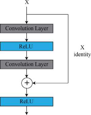
Fig.3. Building block of a ResNet. The input is passed through Convolution layer and the input is added to the output before applying nonlinearity.

One important challenge with the classification of facial attribute comes from the fact that the variations in facial images from one class to another are very small. Tradition models try to optimize categorical cross-entropy loss defined by softmax, which forces the features of different classes by penalizing the misclassified samples. As shown in Fig. 4(a), features are represented in clusters in different feature spaces. However, these are clustered with a bigger area with not much correlation. Also, there is an overlap of different classes because of high inter-class similarities. Recently an additional loss called Center Loss [46] was introduced into CNN to help around this issue. It reduces the intra-class variation and tries to squeeze the features in a smaller area. Still, there might have overlap between different classes. To push the feature space of different class away from one another

Center loss was modified to introduce Island Loss [47]. It increases inter-class distance. simultaneously reduces the intra-class variation and

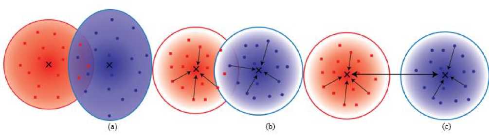
Fig. 4. A visualization of features learned with (a) Only cross-entropy loss, (b) Center loss with cross-entropy loss, and (c) Island loss with crossentropy loss. Adding center loss pushes the features of same class towards its centers which is denoted by the cross sign. With the introduction of Island loss pushed the centers away from one another.

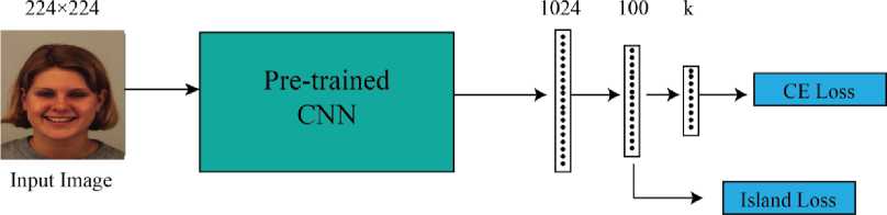
Fig. 5. Proposed model training pipeline. Island loss in the second last fully-connected layer and cross-entropy loss in the final layer. Here, K represent total number of output classes.

This work has approached the facial attribute classification task with pre-trained deep convolutional neural networks with Island Loss. The experiment is conducted on emotion classification and age prediction. The experiment also shows and a comparison of using different pre-trained models in the training process. The methodology section is described with the VGG-16, one popular deep convolutional neural that is used as a running example to illustrate the training process. The training procedure can be used with any other pre-trained models that are used in the experiment. The experiment is conducted on VGG-16 [36], Resnet50, Resnet152 [40], Inception-v3[38], and DenseNet161 [48], which all are very deep CNN models.

The rest of the paper is organized as follow. Section 2 describes the methodology and the custom loss used for classification. Section 3 describes the experimental details. Section 4 compares and discusses the result.

• II.    Methodology

The central concept is to use Island Loss [47] with the transfer learning method as a classifier. The idea of transfer learning is to use a deep pre-trained model as a feature extractor and then train a few of its own layer. The experiments are conducted on Facial Emotion and Age classification task. As the facial images are very similar in different classes of this classification task, the Island Loss is used to separate out the distribution of the features calculated by the neural network. The ImageNet dataset is used in pre-training and it is not strictly related to the facial dataset datasets. The is why earlier layers are fine-tuned to improve the performance. The reason behind such high accuracy can be described by the nature of the deep convolutional neural network. Matthew et al. 2013 [49] showed what CNN layers learn visually. The first layer of the CNN captures basic features like edge, corners of an image. The next layer detects more complex features like textures or shapes. And the upper layer follows the same patterns towards more complex patterns. As these basic features are similar in all images, training in the ImageNet dataset is not a problem for our application.

• A.    Island Loss

As shown in Fig. 4(b), the center loss [46] reduces the intraclass variations between the classes by pushing the features towards the center of all features. The center is updated during training at each iteration and the full model is trained end-to-end.

In the following equation, Lc represents the center loss as the summation of squared distances between features and its class centers.

L_c= 1 SM^-M² (1)

Here yi is the class label of the ith sample. xi is the ith feature representation taken from the output of a fully connected layer of the neural network before the final layer. cy is the center of all feature with class yi and m is the batch size. By minimizing the center loss the variation of inter-class features will minimize by polling the features of same class towards the center.

The combined loss is calculated as the weighted sum of the center loss and the cross-entropy loss.

L = L_s + L_c (2)

Where LS demotes the cross-entropy loss and the L C denotes the center loss. A scalar λ is used to weight the importance of cross-entropy loss and center loss.

As illustrated in Fig. 4(b), introducing center loss reduces the radius of corresponding classes but these classes can have overlap with each other. The objective of Island loss is to reduce the overlap by pushing the centers from each other. This is shown in Fig. 4(c). So, Island loss simultaneously reduces the radius of intraclass variations and increases the inter-class differences.

The Island loss is denoted with LIL, which is defined as the summation of center loss along with pair-wise distances between class centers in features space.

L1L = Lc +Л 1 L^yl^vQ^X Q 2 C. 2 + 1) (3)

Where c k and c j is the k^th and j^th, N is the total number of classes. λ 1 balances the two terms. By minimizing the Island loss the samples of the same class will come closer and the samples from different classes will push further from each other.

The overall loss of the full model is represented as follow:

L = L_s + AL_t L (4)

Where a scalar value λ balances the two losses.

• B.    Feature extraction

In our method, we used the pre-trained model as the feature extractor. The job of the feature extractor is to extract useful features from the given image. The pretrained model can be used as a feature extractor in two ways.

First, using it to generate a low dimensional feature vector from the input image. For such case, no fully connected layer is used on top of the pre-trained model. The pre-trained model block in Fig. 6 shows the feature extractor block. The output of this model is a matrix. In the case of the VGG16 model, the output dimension of the feature extractor is (7, 7, 512). This represents the useful extracted feature of the image. We can do this for all the images in the dataset and store this as a different dataset. This output is then used in a separate model as the input. This model can be a single or two-layer basic neural network. We can train this model on extracted features as input data. This relatively small model on low dimensional data does fairly well. But one disadvantage of this model is that we cannot take advantage of finetuning to improve the pre-trained section of the model. Which is exactly what the next approach does.

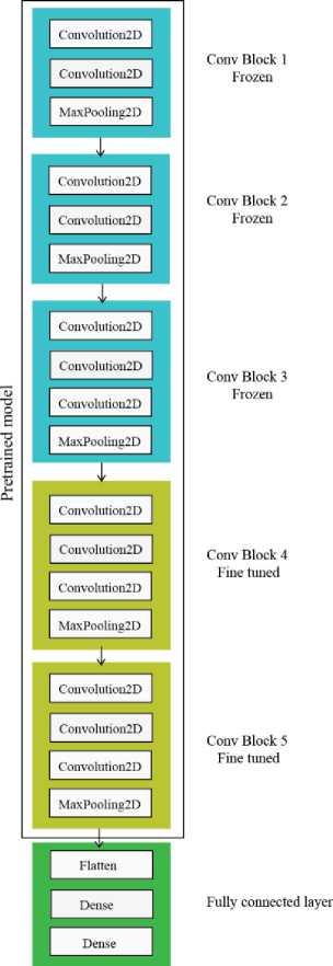
Fig. 6. Architecture of the VGG-16 model. Here pre-trained model section is trained on ImageNet dataset. The fully connected layer is the portion we have added on top of the pre-trained model

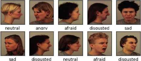
Fig. 7. Sample images from KDEF dataset

Second, we use the model as part of our full model. That means we keep the feature extractor as defined in the main model and add a few new layers on top of that. The green section of Fig. 6 shows the newly added layers. We call this fully connected layer. It is consists of three layers. The first one is a ”Flatten” layer, which converts them into a one-dimensional vector. Two more dense layers are added on top of that. A dense layer is a regular layer of a neural network. It takes some dimension as input and outputs a vector of the desired dimension. The first dense layer is a hidden layer that converts the comparatively higher-dimensional vector into an intermediate-length vector and the final layer takes this as the input. The final layer is also a dense layer that outputs a vector that has the length equals the number of output classes. Here we have 7 different classes of emotional state. The vector represents the probability of the image belonging to each of the classes. Having the full model in the same pipeline gives us the opportunity for fine-tuning some layer with our data. In the first run, we only train the fully connected layer of the model. In the preceding steps, we train one or more block of the pre-trained section. In Fig. 6 yellow represents the blocks that are fine-tuned.

• C.    Fine-tuning

On top of the output of the last layer of the pre-trained model, a Flatten layer is added to convert the 2dimensional metric into a vector. This is followed by dense layers to take it down to 7 classes which correspond to the probabilities of each class. We start the training process by keeping all the layers above this frozen, which are the pre-trained layers. That means we do not change the weights of the model learned from ImageNet dataset and train only the newly added block. This is an important part of fine-tuning. As the newly added layer has random weights at the beginning, in the training process this random weight will generate bad gradient which will be propagated in the trained portion causing deviation from a good result. So, we trained this first to make the weights generate moderately good result then move on to fine-tuning the upper layers. To train more portion of the pre-trained layer we increase finetuning layers slowly instead of training all at a time. It helps diminish the effect of initial random weight and keep a look at accuracy. For the same dataset, a various pre-trained model can give the best accuracy with various amount of layers being fine-tuned. The processing of using the pre-trained model only as a feature extractor and not fine-tuning can do very well if the data is very similar in both applications. But it not the case in our application and we have a very different dataset. For our case, fine-tuning more layers proved to be useful.

• III.    Experiments

We experimented on different model architecture. First we started with the simple convolutional neural network, second, a deep model trained from the sketch, Finally, several deep models pre-trained with ImageNet dataset. We tuned the hyper-parameters for finding the optimal values which include a number of filters, regularization, lining rate, and dropout. We also experimented using batch normalization [50].

• A.    Experimental Datasets

We have conducted experiments on emotion and age classification dataset. For emotion classification, KDEF and JAFFE dataset are used. For age classification task the CACD, UTKface and FGnet dataset is used. Short description of all those datasets is provided below.

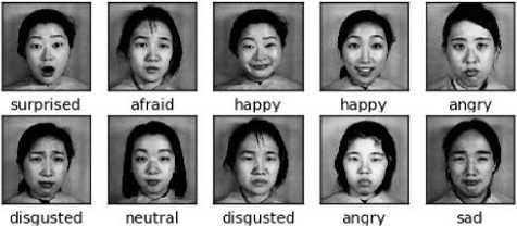
Fig. 8. Sample images from JAFFE dataset

Emotion Datasets

KDEF [51] is a collection of 4900 images which contains 7 emotion class of each person from different angles. The dataset was originally developed by Karolinska Institute, The dataset contains 70 individual people each expressing 7 emotions and 5 photos were taken from 5 different angles.

JAFFE [52] - is a small dataset of the Japanese woman. This is a small dataset with only 213 images of 7 facial expressions. It contains images of some female Japanese models. The dataset was collected by Michael Lyons, Miyuki Kamachi, and Jiro Gyoba. And the photos were taken at the Psychology Department at Kyushu University.

We saw rather than using the raw images provided with the dataset, cropping the images to match the area of the face with a face detection algorithm yield better results. We used the default face detection algorithm comes with OpenCV [53] documented here. (There are other methods of face detection. Viola-Jones method for example. How about V-J method. You need to justify your method.) We trained the model with various input sizes. Larger image size normally does well. The minimal size to use with the pre-trained model is 224 224. With a farther increase in the size of the input, images did not make much change in accuracy. So, in our final model, we used this model we used this image size. In the dataset following acronyms are used. AF: afraid, AN: angry, DI: disgusted, SA: sad, HA: happy, SU: surprised, NE: neutral.

Age Datasets

UTKFace [54] - is a large data set with a long age span and it ranges from 0 to 116. It contains more than 20,000 face images. These images were collected from the internet. It provides the labels in its title i.e. age, gender, race, date and time. We prepared it according to age since we wanted to predict age from images. Given age is an integer number that indicates the corresponding person’s age. These images have lots of variation based on pose, resolution, and expression.

CACD [55] - Cross-Age Celebrity Dataset is the largest data set as far we know. It has more than 160k images of two 2000 celebrities. It also has a large image span with age ranging from 10 to 62. These images were collected from the internet and desired age was calculated by subtracting the birth year from the photo taken a year. Necessary information is given by the image title and it contains age, identity, year, feature, and name. Since we want to map age with a person’s face image we split the data according to the age.

Fig. 9. Sample images from UTKface dataset

Fig. 10. Sample images from CACD dataset

FG-NET [56] - It is a much smaller data set compared to the two described above. This dataset was used here [56]. It contains only 1k images of 63 age group. The necessary information can be obtained from the image name. For instance, 060A12.JPG means Np. 60 persons’ age is 12 years and A is the annotation for Age.

• B.    Experimental setup

  We used Adam [57] optimization algorithm instead of regular stochastic gradient descent. Adam is a recently proposed optimization algorithm that has become very popular in computer vision and natural language processing application. Adam is derived from two optimization- Adaptive Gradient Descent (AdaGrad), which maintains a different learning rate for different parameters of the model. This is good for the sparse gradient. The second one is Root Mean Square Propagation (RMSProp), which also maintain different learning rate and it is the average of previous magnitudes. Adam is derived from adaptive moment estimation. Stochastic gradient descent maintains a single learning rate (termed alpha) for all weight updates and the learning rate does not change during training. It has two momentum parameter that adjusts the learning rate decay. It calculated gradient based on an exponential moving average which is control by the value of beta1 and beta2. Here beta1 and beta2 are exponential decay rate of first and second-moment estimates. The parameters of the optimizer are- Learning rate: 0.0005, Beta1: 0.9, Beta2:0.009.

• C.    Data augmentation

Data augmentation is a process of making more data from the available data. It is a very effective technique for image data. In this case, new data is generated by rotating, shifting or flipping the original image. The intuition is that if we rotate, shift, scale or flip the original image this is still the same subject but the image is not the same as before. By this process, we can generate more data from the given data. It is embedded in the Dataloader in the training. Every time it loads the data from memory a small transformation is applied to the image to generate a slightly different data. As the exact same is not given to the model the model is less prone to over fittings. This is very helpful especially when the dataset is not very large which the case for our model is. In our particular application, we used carefully tuned augmentation. As we have all image perfectly cropped in each size we did not apply rotation to the image. We only used slight transformation and scaling with horizontal flipping. Applying a small transformation to the original image increased our accuracy of around 2-3% with this augmentation the new cost function of our model to considering all images is:

loss =

N T

- 22 logP(yn|n£n)

n=1 t=1

Where N represents the number of images in the dataset and t is the number for transformation to perform over an image. In code, we, however, don’t have to create the augmented dataset beforehand. We applied the random transform to the batch of images selected for each epoch from t possible combination of transformation.

As the images of our dataset are nicely collected we carefully applied only a little amount of augmentation. The augmentation settings are Rotation: (-10 to 10), scaling factor: ×1.1, Horizontal Flip.

Island Loss settings - The equation of island loss has two hyper-parameters. We experimented with different values of λ and λ1. The optimal values found for λ = 0.25 and λ1 = 0.1 is used for rest of the experiments.

• IV.    Results

• A.    Emotion classification task

Before we experiment on our model we built a basic 2-layer convolutional neural network to find a baseline accuracy. We conducted several experiments with some hyperparameters and regularization techniques. The accuracies of different experiments are given in the table below.

Table 1. Accuracies on Different Input Size Images On 2-Layer CNN with KDEF And JAFFE Dataset

Input size	KDEF	JAFFE
360 × 360	73.73%	91.67%
224 × 224	73.34%	87.50%
128 × 128	80.35%	91.67%
64 × 64	69.33%	83.33%
48 × 48	61.91%	79.17%

As we can see from the result of the model above, it gives the best accuracy with the image size of (128×128) and the accuracy decreases with a bigger image. Although a bigger image more information and should do well the better classify the images, the small model cannot do well with large data. The reason is that it does not have enough parameters to fit the high dimension data and training more result in over-fittings. This is way bigger models are needed.

As we discussed in the method, we conducted an experiment on the pre-trained model. First, we experimented on the VGG-16 model. We first trained the fully connected layer then we fine-tuned different portion of the model to see the effectiveness of fine-tuning the pre-trained layers. The accuracy of a model varies in training mode depending on the data and the amount of data. Less data like JAFFE dataset cannot tune very large network top to bottom but with more data, training more layers can help to improve the accuracies. The table below summarizes the accuracies in different training settings on this model. Here fc stands for the fully connected layer.

Table 2. Comparison of accuracies on different training mode of VGG16 on KDEF and JAFFE dataset.

Training	KDEF	JAFFE
Vgg-16 fc layer only	77.73%	91.67%
fc + Vgg-16 last block (block-4 )	91.93%	95.83%
Full Vgg-16 model	93.51%	100.0%

The observation from the table concludes that the best way to use the proposed pre-training approach with the pre-trained model is to train the full model. In this case, we have gradually increased the number of layers we want to fine tune. Staring training of the random initialized alyers onf the top and the pre-trained layers might change the layer weight in a bad direction that will be difficult to recover. For rest of the experiments we have used the full model fine-tunning approach.

Now we have conducted an experiment on all mentioned models. As we can see the deeper and bigger models are giving better accuracy than the shallow ones. The table below shows the accuracies on all models.

Table 3. Comparison of the accuracies with different pre-trained model in KDEF and JAFFE dataset.

Pre-train model	KDEF	JAFFE
Vgg-16	93.51%	100.0%
Vgg-19-BN	96.76%	100.0%
resnet-18	95.54%	100.0%
resnet-34	96.03%	100.0%
resnet-50	97.57%	100.0%
resnet-152	96.71%	100.0%
Inception-v3	97.57%	100.0%
Densenet-161	98.84%	100.0%

The exeperiments with 2 variations of VGG, 4 fariations of ResNet, Inception and DenseNet models shows the best performace of both model with DenseNet-161 network. So, we have considered this as a go to model for rest of the general purpose experiment.

We have calculated per class accuracy to see the classification rate of each class. We represented this in a table to see which class is classified as which.

Table 4. Accuracies of each emotion class KDEF and JAFFE dataset.

Emotion	Accuracy (KDEF)	Accuracy (JAFFE)
Afraid	98.1%	100.0%
Angry	98.7%	100.0%
Disgust	98.5%	100.0%
Happy	99.4%	100.0%
Neutral	99.2%	100.0%
Sad	98.8%	100.0%
Surprised	99.1%	100.0%

From the table above we see that the proposed model generalizes over all the emotion classes without much bias towards any of the classes, which is a good sign for any classification model. Following is the confusion metix over all the classes of the dataset.

Table 5. Classification of each emotion class of KDEF dataset with 235 test images

	AF	AN	DI	HA	NE	SA	SU
AF	30	0	0	0	0	1	1
AN	0	39	0	0	0	0	0
DI	0	0	37	0	0	0	0
HA	0	0	0	36	0	0	0
NE	0	0	0	0	25	0	0
SA	1	0	0	0	0	30	0
SU	0	0	0	0	0	0	35

From the confusion metrix we can see that apart from 2 classes all the other class has no errors on the test dataset to classify properly. The ‘Sad’ and the ‘Surprised’ classes has a total of 3 miss-classified examples.

The JAFFE is comparably an older dataset and a good amount of research has used this dataset to handle the emotion recognition problem. Here is the comparison of the accuracy of our model with known previous works.

Table 6. Comparison with previous methods on KDEF and JAFFE datasets.

Approaches	KDEF	JAFFE
2-layers CNN	80.33%	91.67%
CNN with regularization	82.17%	92.88%
Qi and Jiang [58], 2007	-	94.64%
Feng et al. [59], 2007	-	93.8
Zhao et al. [60], 2008	-	93.72
Zhi and Ruan [61], 2008	-	95.91
Shin et al. [62], 2008	-	95.7
Chang & Huang [30], 2010	-	98.98
Shih et al. [9], 2012	-	96.43
Liew et al. [63], 2015	82.4%	-
Alshami el al. [64], 2017	90.8%	91.9%
Our proposed method	98.93%	100.0%

The accuracy on JAFFE has beaten all previous results and got 100% accuracy. So, there is no room for improvement. But the KDEF was a little more challenging one and we tried very deep models to improve the accuracies and we experimented with Island loss to improve the accuracy.

Now we show the comparison of the proposed loss with the standaed categorical cross entropy loss. As methioned in the method, the Island loss combies the objective of regular categorical loss along with the pinalization of classification precision.

Here is the comparison of the accuracies with crossentropy loss and Island loss.

Table 7. Comparison of the accuracies with different pre-trained models with Cross-entropy loss and Island loss on KDEF dataset.

Pre-train model	Accuracy (CE-loss)	Accuracy (Island-loss)
resnet-18	95.54%	97.57%
resnet-34	96.03%	97.57%
resnet-50	97.57%	98.38%
resnet-152	96.71%	97.57%
Inception-v3	97.57%	98.38%
Densenet-161	98.84%	98.96%

As we can see from the comparison, even smaller model like ResNet-18 has an improvement of 2% of accuracy. All other model has gone through some improvement with the introduction of Island loss.

There are few hyper-peremeters associated with the proposed loss function. We conducted experiments to find the optimal values for those parameters. The following table summarizes the performance of the model with the change in the values of the hyper-parameters.

Table 8. Accuracies of each emotion class on KDEF and JAFFE

λ	λ 1	Accuracy
0.1	1.0	97.14%
0.1	0.1	97.31%
0.25	0.025	96.76%
0.25	0.1	97.57%
0.5	0.1	97.46%
0.5	0.025	97.31%

We conducted experiments to find the optimal values of λ and λ 1 on ResNet-18 model. Following the outcomes of the model with different values of these hyper-parameters.

• B.    Age classification task

Table 9 and 10 show the classification results on the datasets CACD and UTKFace accordingly. Here we used three metrics for describing our results, they are accuracy, 5 class off and 10 class off. As mentioned earlier age classification task isn’t the same as other classification tasks in real life because age class has some coherence unlike other classification tasks i.e age pattern of 31 and 33 years old person’s may be similar and even human eye may differentiate a little. So, we decided to off 5 classes and 10 classes off and introduced a different metric.

We Summarize the experiment with the CACD dataset in the following table.

Table 9. Classification results of CACD

Methods	CACD
	Acc	5 Class	10 Class
ResNet18	10.21%	71.37%	90.60%
ResNet34	10.33%	71.78%	89.68%
ResNet50	15.11%	72.12%	90.01%
Inception-v3	40.09%	80.75%	92.12%
DenseNet	58.78%	85.97%	93.11%

The table above shows the best performance if all measurement in DenseNet model. For these model, appart from the 10 class distance consideration all other are far off from the DenseNet accuracy.

The experiments with the UTKFace dataset is summarized in the following table.

Table 10. Classification results of UTKFACE

Methods	UTKFace
	Acc	5 Class	10 Class
ResNet18	89.83%	95.85%	98.23%
ResNet34	68.25%	89.93%	96.19%
ResNet50	89.12%	97.52%	99.02%
Inception-v3	43.22%	82.26%	93.35%
DenseNet	76.82%	94.21%	99.34%

Unlike the CACD dataset, the best formance model is different for different measurement. The DenseNet still performes the best for 10-clas off case. But for direct accuracy and the 5-class off case the ResNet50 performs comperativelty better.

Next we compare the result with and without the proposed loss in the age classification task. Following table summarized the results.

Table 11. Comparison of the 10-class-off accuracies with different pretrained models with cross-entropy loss and island loss on UTKFace dataset

Pre-train model	Accuracy (CE-loss)	Accuracy (Island-loss)
resnet-18	98.23%	99.02%
resnet-34	96.03%	97.57%
resnet-50	97.57%	98.38%
Inception-v3	97.57%	98.38%
Densenet-161	98.34%	99.39%

Similar to emotion classification task we have found improvement in age classification with the introduction of Island Loss with softmax loss.

Finally, the result is compared with previous work to evaluate the performance of the model on the age classification task. More previous works have used FGnet dataset and reported the performance in mean square error (MSE). The table below shows the result in comparison with previous works on FGnet dataset.

Table 12. Comparison on MAE with other methods on FGNET dataset

Method Name	MAE
Geng et al. [23]	6.8
Suo et al. [65]	4.7
Guo et al. [21]	4.8
Luu et al. [66]	4.1
Chang et al. [67]	4.5
Wu et al. [68]	5.9
Thukral et al. [69]	6.2
Chao et al. [70]	4.4
Our Proposed Method Using ResNet34	2.5

As we can see from the table above, the proposed model does significantly better than the previous results in age classification task also.

• C.    Effects of noise

We introduced a few noise function to generate a noisy version of test data and observed how the accuracy changes with an introduction to noise and other effects on the image which might be the case of real-world data. We found that if the noise condition is not very extreme the model holds good, and the accuracy does not fluctuate more than 3-4%. The accuracy of each class of emotion on each noise data is given in the table below.

Table 13. Accuracy change with the introduction of noise on KDEF

Noise type	Accuracy
Original	98.8%
Salt and piper noise	94.4%
Gauss noise	95.5%
Poisson noise	96.1%

Our proposed model is regid enough to perform quite well even with the introduction to different noises. The accuracy does not fluxtuates more that 2/3% with this. Next we present perclass accuracy of the model when noise in introduces to the images.

Table 14. Classification of each emotion class of kdef dataset with 235 test images

	AF	AN	DI	HA	NE	SA	SU
Original	98.1	98.7	98.5	99.4	99.2	98.8	99.1
Poisson	82.9	97.1	89.9	99.9	97.1	86.2	92.1
Gauss	81.2	97.1	89.6	98.5	97.8	86.1	92.1
Salt piper	77.9	97.9	82.6	95.6	89.7	85.3	89.9
Speckle	6.7	73.1	41.0	3.6	3.7	37.1	0.1

Only very extrem loss casues problem to the model. Other than that all other modes have fair performance with the introduction to different loss.

From the result above, we can conclude that our model is very robust and perform quite well with most of the noises added to the image.

• V.    Conclusion

This work proposed the use of the pre-trained model for facial attribute classification task along with the island loss to help better classify the extreme similarities in between classes. Classifying different facial attribute has many different real-world applications. We have experimented on two different tasks with several datasets to examine the effectiveness of the proposed model and got comparatively improved results in both cases. From the result, it can be concluded that the accuracy of any classification can be improved with this custom loss where the similarities in between class are high and the rate of improvement is high with a lower number of classification class.