Исследование тензорной анизотропии космических лучей во время крупномасштабных возмущений солнечного ветра

NATURE OF ANISOTROPY

An anisotropic flow of cosmic rays (CR), which is registered by ground-based detectors, is originated first of all from dynamic processes in the solar wind, which affect CR through the interplanetary magnetic field (IMF). Notice that CR anisotropy also occurs outside the heliosphere, but for the particles registered by ground-based CR detectors, the solar wind is the main modulation factor. The observed anisotropy can be presented by the first two spherical harmonics expressing themselves as diurnal variations due to the Earth rotation. In the angular coordinate system, with the polar axis parallel to the axis of the Earth rotation, the first spherical harmonic is presented as a component R ₁ ¹ . This component can be represented as a vector and is called vector anisotropy. R ₁ ¹ reflects a direct motion or current of CR. The current has a convective or diffusive origin. The convective current appears when CR move together with the solar wind magnetic field; and the diffusive current, due to CR gradients and their scattering by magnetic irregularities. In the steady state of the interplanetary medium, the convective current is directed away from the Sun; and the diffusive current, toward the Sun along IMF lines. In general, the diurnal anisotropy shows the moment of maximum intensity about 18 LT.

The tensor anisotropy components R22 and R21 in the above angular coordinate system appear as semidiurnal and antisymmetric diurnal variations. The reason for the observed anisotropy R22 is a deficit of particles moving along field lines in loop structures of IMF. In average over the course of a long period, this component is presented, on the 12-hour dial, as a vector directed to 3 LT. The same anisotropy should appear in the presence of the heliolatitudinal CR gradient with minimum intensity near Earth’s heliolatitude. A deviation of magnetic tubes from the Archimedian spiral leads to a change of the R22 direction. The component R21 usually appears in the region of heliolatitudinal shift of the CR current. If the convective current shifts, then R21 is maximum at 12 or 0 LT. If there is a heliolatitu-dinal shift of the diffusive current along the field lines, the variation is maximum at 9 or 21 LT. In more complicated cases, when the convective and diffusive currents shift simultaneously and when field tubes are deviated, the tensor anisotropy behaves in a complicated way.

THE METHODOF STUDYING ANISOTROPY

Variations in CR density and anisotropy observed during the passage of large-scale SW disturbances through Earth have been extensively studied, for example, by the following groups of researchers: the IZMI-RAN group using their version of the global survey method (see, e.g., [Belov et al., 2009; Abunina et al., 2015; Abunina et al., 2013]), the ISTP group using the original method of global spectrographic survey [Kravtsova, Sdobnov. 2016] and the group of Japanese researchers [Munakata et al., 2005]. The version of the global survey method employed by the IZMIRAN and Japanese groups is largely similar to the method developed in ShICRA and used in this work. However, the above works ignore the second spherical harmonic. The method of global spectrographic survey employed by the ISTP group has a slightly different way of presenting CR angular distribution. Thus, at present, ShICRA’s method of global survey is one of the most effective methods for studying short-term CR variation.

Information about CR angular distribution has been obtained using data from the worldwide network of neutron monitors with the global survey method [Altukhov et al., 1970]. Below is a brief description of the method.

The observed CR intensity J (θ, ϕ ) can be represented as a series of spherical harmonics by the equation:

∞ n

J( θ , φ )= ∑ ∑ ( a_n^m cos m φ +b_n^m sin m φ) P_n^m (sinθ) , n= 0 m= 0

where θ, ϕ are latitudinal and longitudinal angles respectively, P_n^m is the associated Legendre polynomial. So, the angular distribution has the form of the multidimensional vector A = ( a_n^m,b_n^m ), where 0 ≤ m ≤ n< ∞ .

Since the registered particles are affected by the geomagnetic field, the intensity registered by a CR detector J =A ⋅ Z , where Z = ( x_n^m , y_n^m ) is the multidimensional acceptance vector, which accounts for the directional diagram of a device, coupling coefficients, particle trajectories in the geomagnetic field, etc. [Grigoryev et al., 2011].

Given that each neutron-monitor detector has different energetic sensitivity, it is necessary to enter an additional spectral multiplier K_n^j , which normalizes j -th device readings to a device with the coupling coefficient W 0 ( ε ):

∞

∫ Wj (ε)fn (ε)dε j    emin

K= , n _∞

∫ W0(ε)fn (ε)dε emin where fn(ε) is the energy spectrum of n-th spherical harmonic (energy spectra of the first two spherical harmonics are presented in [Grigoryev et al., 2011]). Using data from all the j devices, we solve the system of equations:

∞∞

J j = _∑∑ (a_n m ,0 x_n m,j +b_n m,0 y_n m,j )K_n j , n= 0 m= 0

where a_n^{m ,0} , b_n^{m ,0} are unknown components. Thus, with a sufficient number of neutron monitors it is possible to obtain hour-to-hour changes of CR angular distribution. Notice that with the available number of active neutron monitors we can consider only the first two spherical harmonics as higher harmonics have insufficient accuracy.

The component a00 represents an isotropic intensity. The first spherical harmonic consists of the first zonal a10 and azimuthal a11,b11 components; the last two com- ponents describe a symmetrical diurnal variation of CR. The second spherical harmonic comprises the following five components: second zonal a20 , antisymmetric diurnal a12, b12 and semidiurnal a22, b22 variations. The first and second spherical harmonics can be represented in space as a vector and tensor and are called CR vector and tensor anisotropy respectively. For convenience, we designate each pair of components anm, bnm as Rnm .

It is well known that during periods of passage of large-scale SW disturbances through Earth strong geomagnetic storms occur which can change geomagnetic cutoff rigidities of CR; hence calculated receiving vectors differ from real ones. However, a large number of selected neutron monitor stations, which are uniformly distributed over the Earth surface, can neutralize this effect.

EXAMPLESOF FORBUSH DECREASE EVENTS

To analyze the behavior of the above components during a passage of large-scale SW disturbances, we have chosen two time periods with large Forbush decreases (FD): November 2001 and November 2004. The total number of neutron monitor stations used for the events of interest is equal to 27, which is quite enough to obtain the first two harmonics of CR angular distribution with a high level of accuracy.

Information about FD and their sources are obtained from the catalogue created by Zhang et al. [Zhang et al., 2007]. This catalogue contains data on probable sources of 88 major geomagnetic storms that occurred in 1996–2005. In particular, it identifies times of arrival of the disturbances in Earth, coordinates of the respective solar flare, and the type of the interplanetary solar wind structure.

Two large FD with amplitudes of ~10 % and ~7 % respectively were registered by high-latitude neutron monitor stations on November 6 and 24, 2001. The source of the November 6 FD was a solar flare in the active region AR9684 with coordinates (06° N, 18° W) and the source of the November 24 FD was a flare in AR9704 with coordinates (14° S, 36° W). On November 7 and 9, 2004, two FD with amplitudes of ~5 % occurred. The probable source of these FD is the active region 10696 with coordinates (09° N, 17° W), which was accompanied by multiple solar flares of class up to X2.5.

To get a complete picture of the relationship between CR anisotropy and specific physical processes, Figure 1 presents SW parameters (solar wind speed Vsw, IMF Bx, By, Bz components, SW flow pressure, and SW proton density), obtained from the OmniWeb database [King, Pa-pitashvili, 2005]. Moreover, this Figure shows values of the first R10 and second R20 zonal harmonics and isotropic intensity dI, which were obtained with the global survey method. Red vertical lines indicate the moments of arrival of the disturbed solar wind in Earth. These moments were determined from catalogues presented in

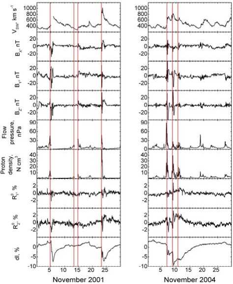
Figure 1. Parameters of IMF B x , B y , B z , solar wind speed V sw , flow pressure and proton density, first R ₁ ⁰ and second R ₂ ⁰ spherical harmonics and isotropic intensity dI in November 2001 and November 2004

[Jian et al., 2006] and [Zhang et al., 2007]. The beginning of the isotropic intensity decreases on November 5 and 24, 2001 was followed by abrupt increases in the solar wind speed, flow pressure, proton density, and IMF intensity. At the same moments, there were R ₂ ⁰ decreases with a value of ~2.5 %. Note that maximum R ₂ ⁰ decreases have always occurred at maximum solar wind speed and short-term increases in the IMF B z component. The above mentioned relationship of R ₂ ⁰ with the solar wind parameters was also observed during FD in November 2004. As for R ₁ ⁰ , it has not a sufficiently reliable response.

The R ₁ ¹ , R ¹ ₂ , and R ₂ ² components are presented on a vector diagram (Figures 2–4) as linked vectors which form a continuous curve. The numbers near the curves indicate days of the month; red triangles mark the time moments of ICME arrival in Earth.

The behavior of the vector anisotropy component R ₁ ¹ during FD in November 2001 and November 2004 is illustrated in Figure 2. Notice that at the end of the previous month, October 28, according to [Zhang et al., 2007] ICME arrived in Earth. It is clearly seen that during the phase of CR intensity decrease, the arrival of the disturbed solar wind, the convective current of CR prevails; and during the recovery phase, the sunward diffusive current of CR along IMF predominates. It is necessary to note here that if a solar wind disturbance passed

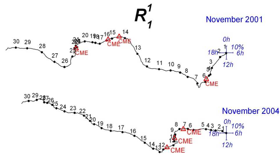
Figure 2. Behavior of R ₁ ¹ in November 2001 and November 2004

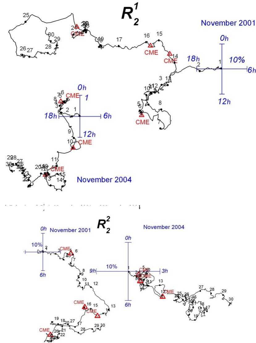
9h

Figure 4. Behavior of R ₂ ² in November 2001 and November 2004

Figure 3. Behavior of R ₂ ¹ in November 2001 and November 2004

close to but away from Earth, we would expect the appearance of an antisunward diffusive current of CR in Earth against a quiet solar wind. But in this work, given that large-scale FD occur with abrupt SW increases, it is fair to assume that Earth is in the central disturbed region and the antisunward CR current should be convective.

Figures 3 and 4 present the tensor anisotropy components R ₂ ¹ and R ₂ ² . It is obvious that these components experience much more complicated variations as compared to R ₁ ¹ .

The leading front of the disturbance was observed on November 5 and 6, 2001. It was accompanied by disappearance of R ₂ ² that was earlier directed to 3 LT. In the recovery phase of the disturbance, from November 4 to November 14, the component R ₂ ² shifted toward 5 LT. This suggests some straightening of the Archimedian spiral during this period. The component R ¹ ₂ on November 5 and 6 almost disappeared and then recovered with a direction at 22 LT. This may mean that the diffusive current increased in southern heliolatitudes.

The solar wind disturbance on November 23 and 24, 2001 occurred with a significant decrease in R ₂ ² and its subsequent recovery with a direction at 3 LT. The component R ¹ ₂ behaves itself in a complicated way, revealing a large CR current shift in the main phase of the disturbance.

The event in November 2004 is an interference of multiple high-speed flows with a maximum on November 8. From November 8 to November 11, the component R ¹ ₂ revealed a convective current increase in northern heliolatitudes. As for R ₂ ² , this component does not show significant changes caused by the disturbance.

As inferred from [King, Papitashvili, 2005], FD on November 5, 2001 occurred due to the arrival of multiple solar wind structures (magnetic cloud, ICME, and shock wave) in Earth. The November 24, 2001 FD was caused by multiple shock waves and ICME. On November 7, 2004, multiple shock waves and a magnetic cloud entered the interplanetary space; and on November 9, a magnetic cloud and ICME. Thus, in our selected FD events there were always different solar wind structures. This fact explains the observed ambiguity of the tensor anisotropy behavior during these FD events. The behavior of tensor anisotropy strongly depends on the solar wind structure. To clearly determine the CR anisotropy behavior during different solar wind disturbances, it is necessary to conduct a more detailed investigation with a great number of data.

CONCLUSION

The analysis of the behavior of CR angular distribution during FD events in November 2001 and November 2004 allows the following preliminary conclusions:

• •    arrival of solar wind disturbed structures in Earth is accompanied by abrupt decreases in the second zonal harmonic R ₂ ⁰ . The component R ₁ ⁰ does not reveal such big changes;

• •    during the phase of CR intensity decrease, the convective current of CR predominates; during the recovery phase, the sunward CR diffusive current along IMF dominates;

• •    the components of tensor anisotropy R ₂ ¹ and R ₂ ² during passage of large-scale disturbances of solar wind experience complicated amplitude-phase variations. To clearly determine the observed variations of the tensor anisotropy, it is necessary to conduct further more detailed investigations.

The work was supported by RFBR grants Nos. 15-42-05085-r_vostok_a, 15-42-05083-r_vostok_a and by RAS Presidium Fundamental Research Program No. 23 “High-energy physics and neutrino astrophysics”.