Iterative Shrinkage Operator for Direction of Arrival Estimation

Published Online September 2016 in MECS DOI: 10.5815/ijieeb.2016.05.04

Array processing uses array of sensors for sensing and/or spatial filtering. Arrays find extensive applications in defense, medicine, seismology, communication, oceanic studies etc. Direction of arrival estimation (DOA estimation) is one of the key processing tasks in arrays [1].

DOA estimation concerns itself with locating peaks in spatial domain, corresponding to radiating sources' location. DOA estimation techniques can broadly be classified into parametric and non-parametric techniques. Non-parametric techniques make no assumption about the functional form of directional power spectrum. Beam scan, MVDR (Minimum variance distortion less response/CAPON beam former), LCMV (linearly constrained minimum variance) are major examples of non-parametric DOA estimation [2].

Parametric techniques, on the hand, assume some function form of spatial power spectra. Parametric techniques usually have high resolution and more robust then non-parametric techniques. The benefits however come at the cost of computational complexity. Min-norm, WSF (weighted subspace fitting), MUSIC, ESPIRIT and ML based techniques [3].

There has been active research in application of soft computing techniques to approximate the ML solution. ML solution is the most accurate but is computationally intractable. Hence there has been an active research in approximating the solution around local maxima with accurate initialization techniques. Ant colony optimization, Genetic algorithms and other techniques have been used for DOA estimation [4].

Recently there has been an explosion of interest in compressive sensing paradigm. New algorithms surface almost daily for recovering signals using essentially information rate sampling followed by sparsity promoting based processing [5].

Compressive sensing techniques rely on the dimensionality reduction of the system in alternate basis. For example, an image usually has few significant coefficients in its wavelet transform. This is the basis of jpeg2000 standard [6]. CS techniques directly uses the over-complete basis which can sparsely represent the system. Once such a setup is in place we call upon the methods to recover the solution using sparsity promoting norms, which restricts solution of the otherwise overdetermined system [7].

Generally speaking CS based techniques can be divided into norm approximation, greedy methods, iterative shrinkage operators and Bayesian techniques. Amongst these, first three techniques are due to the fact that norm preferred for measuring solution sparsity, the l o norm based solution is NP hard problem [8].

In norm approximation technique l o norm is replaced by l _p norm with p<=1. With p=1 the optimization problem is convex and easily amenable to variety of standard solvers. Basis Pursuit is one of the popular example of l 1 norm based solution . solution based upon l p norms with p<1 are investigated in [9] .

Greedy methods approximates solution rather than problem statement. The greedy methods update solution set one basis vector at time until the solution set approximate the solution. OMP is a popular example of this class of techniques [10].

Iterative shrinkage operators are similar to greedy methods. Instead of adding a single basis vector at each iteration IS operator uses principle of shrinkage to add multiple solutions to the set at each iteration. StOMP is a popular algorithm in his class [11].

Bayesian techniques in CS employ priors that promote sparsity. Gaussian prior is a popular choice. GSM priors have also been used in [12]. There is tremendous variety of techniques in BCS with different priors, approximation techniques and solution set construction techniques. RVM is a popular choice in BCS techniques[13].

In this technical correspondence we report application of one such compressive sensing paradigm, commonly known as iterative shrinkage operator. A particular algorithm belonging to this general class, the StOMP is employed for application to DOA estimation. Results are compared to MUSIC, which is the state of the art in DOA estimation [3].

Application of CS techniques to DOA estimation is an active research area. In [14] authors have applied l 1 optimization with custom interior point solver. In [15,16] Bayesian compressive sensing is applied to the DOA estimation. In [12] GSM priors are used in Bayesian Compressive settings, in [15] RVM is used for DOA estimation, [16] has used MSBL and TMSBL for DOA estimation.

All these applications are empirical studies. The CS regime employs sensing matrices with particular structure [1]. These matrices can be analytically analyzed to give some measure of Restricted Isometry (RIP) constant [17]. This, in turns gives bounds on recovery performance of the particular CS algorithm.

DOA estimation employs spatially discritised array steering vector as sensing matrix [18]. This particular matrix has not been amenable to analytical measures [19]. This warrants the empirical study of variety of CS algorithms to the DOA estimation problem. Under such assumptions, when sensing matrix is not of standard structure, performance of particular algorithm cannot be gauged. This is the reason for such active research in this particular area.

Iterative Shrinkage operators are particular instance of CS algorithms. The IS operators are characterized by their high speed and computational efficiency. In large problem setting, like medical imaging, such characteristics are particularly useful. This is the particular setting that has been used for application of IS operators [20].

A particular instance of IS operator is StOMP (Stage wise Orthogonal Matching Pursuit) have been employed to find solution of sparse problems. However this has been attempted for large settings with limited scenarios, dictionaries [20]. This lack of analysis has led to this research. DOA estimation employs deterministic dictionary that has coherence. This warrants analysis of IS operators on this scenario.

MUSIC is a parametric technique that uses concept of subspaces. It assumes that a signal space is row space of the steering matrix whereas noise lies in the null space or column space of the array steering matrix. The null space and row space are orthogonal complement for a full rank matrix [21].

MUSIC uses orthognality of noise and signal subspace to locate peaks in spatial spectrum. It computes numerical inverse of the noise subspace. Orthognality leads to nulling of noise subspace at the signal location which gives a sharp peak at that location. Under certain conditions, it's an ML estimate of the actual spatial spectrum [22].

This paper is organized as follows. Section I gives introduction. In section II we discuss the data model. In section III we present details of MUSIC and StOMP algorithms. Section IV details the simulation setup. In section V we give simulation results. Section VI concludes the paper and proposes future direction for the research.

• II.    Data Model

In array processing multiple sensors receive time delayed copy of the same signal. It is the phase difference induced by the time delay that enables array to fix the direction of incoming source.

If we have signals from multiple sources then these signals can be represented as a column vector. The signal received by each sensor is phase shifted version of each other. The phase shifting is mathematically represented as multiplication by complex exponential whose exponent is a nonlinear function of signal bearing, inter element spacing, distance of the sensor from phase center of array and wavelength of the signal.

This weighting is done for each sensor and each source. For single source and L number of sensors we have

L м t)=£ e (O ■л-d) ^( t) i=1

Same procedure is repeated for all the other sources and array output is taken to be the sum of outputs due to all signals.

Mathematically this operation can be conveniently summed up in vector-matrix notation and is given as.

y = Ax + n              (1)

Where;

y = Output of the array.

A = Array steering matrix of dimensions M x L , made up of array steering vectors in directions of sources i.e.

A = [a(6-1)a(O^)            a(0l)]

a (O ) = Steering vector corresponding to i^th source.

L =Number of sources.

M = Number of sensors.

x = Source signal vector.

n = noise.

Direction of arrival estimation is generally concerned with estimation of A matrix.

In this paper we assume a linear array with isotropic elements. Inter-element spacing is constant. Narrowband model is assumed and spacing value is fixed at λ /2

Mostly, techniques estimate the whole spatial spectrum. From this spectrum the peaks give the direction of sources. This is usually done by steering the beam in all directions, noting the received energy. Thus the data model for most of the techniques would use the received signal to form data covariance matrix and then use some form of relation between data covariance matrix and array steering vector in each direction [23].

Compressive sensing, on the other hand implicitly defines matrix to be composed of sampling of all possible steering vectors. Thus, for compressive sensing

jkt»nt -90")          ^yArf,.«_H(-89⁰l                gjkd^i 90°)

Where assumptions made earlier about array are employed.

Spatial spectrum is a continuous function. Discretisation of spatial domain lead to grid errors [24]. Grid errors are due to the fact that actual source lies in between two grid points rather than on a particular point. In [14] grid error is mitigated using multi-resolution refinement whereas in [16] the algorithm itself is robust against grid errors. Further in reference [25] discretisation errors are analytically formulated. Nevertheless it is an active research area and grid errors are part and parcel of the CS regime.

Scanning is performed only in azimuth with array bore sight is at 0o. With A extended to include all possible directions, the signal vector is also extended with zeros where no signal exist; hence, x = [0.x0. „0.x . „0.xL „ .0]

This gives us following data model for compressive sensing [26], y = Ax + n            (2)

In next section, when we present details about the algorithms, we would see that this difference in data model is one of the primary differences in compressive sensing and traditional techniques.

• III.    The Algorithms

In this section we give brief description about algorithms

• A.    MUSIC (Multiple Signal Classification) Algorithm

MUSIC algorithm exploits the geometrical description inherent in Pisaranko’s signal decomposition. In harmonic decomposition, the signal can be thought of as a component in multi-dimensional space whose bases are composed of complex exponentials. These bases are Eigen vectors of covariance matrix of the data which is to be decomposed.

Harmonic decomposition of a signal with noise, hence has a particular structure. Eigen values corresponding to noise form an orthogonal subspace to that of signal subspace. In this section MUSIC algorithm is derived.

Consider the signal model given by (1)

y = Ax + n

A = [ a 9 ) a ( 9 2) a (9l )]

x = [ x₀.

.. x.. X l ^]

For uncorrelated signals we define data covariance vector as;

R = E { yy H }

= E { Axx H A H } + E { nn ^H }

= ABA H + 7 ² I

= Rs + 7 2I

Where,

R_s = ABA H:

"e {|x0|2 }      о      -      0"

B= 0    £(N2} ;•

;                       о о о ••■ e {|xj2 }

Structure of array steering matrix A and data covariance matrix B dictates that there must be L Eigen values corresponding to sources. While remaining M — L Eigen values correspond to noise ( M > L is implied). Based on this premise MUSIC spectrum is given as,

PMUSIC (⁹ ) =

Z M— ^L a H ( 9 ) q. ? ²

a H (9) QnQHa (9)

= Q H a ( 9 )²

Where;

q = i ^th Eigen vector associated with noise subspace.

Q = m atrix composed of q .

Here orthogonality of signal and noise subspace has been exploited. Whenever there is signal present the corresponding steering vector is orthogonal to and denominator becomes zero giving a sharp peak.

Q_n is made of M — L smallest eigenvectors of R .

This derivation is based on [22].

• B.    StOMP (Stage Wise Ortogonal Matching Pursuit) Algorithm

StOMP is a CS algorithm that belongs to iterative shrinkage type of operators. Such class of algorithms typically adds multiple bases to the solution set per iteration. The decision as to which bases should be added is done via shrinkage operator.

Characteristics of shrinkage operator in essence define the characteristics of a particular algorithm. In StOMP multiple access interference cancellation technique of wireless communication and RADAR is carried over to IS operator.

Shrinkage operator operates by defining a threshold and then selecting all bases values whose similarity index exceeds the selected threshold. In StOMP threshold can be computed by either considering false alarms or missed detection rate. Details of the procedure follow in this section.

Consider data model given in (2).

y = Ax + n

A = [ a ( - 90 0 )   a ( - 89⁰)  ......... a (90⁰)]

x = [0„x0. „0.x . „0.xL. „0]

Such a model is amenable to sparsity promoting optimizations, generally given as;

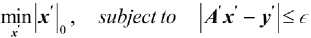
Optimization problem posed in (5) is combinatorial in nature and as such is intractable. Various techniques exist to solve the optimization e.g. [27]. Amongst these, greedy methods have found widespread use [5]. Iterative shrinkage (IS) operators belong to such greedy methods.

IS techniques recursively estimate the solution by computing resemblance of residual with over complete dictionary/basis, adding the resemblance to the solution set, reconstructing the current solution using this set and estimating the residual. This procedure is iteratively applied until number of iterations or the error in reconstruction reaches threshold. Fig. 1 explains this iteration.

initialization

,    ≜        ,   =

Resemblance operation Solution set update Computing solution Residual computation

≜

⨀ ≜

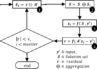
Fig.1. General principle of Iterative Shrinkage Algorithm

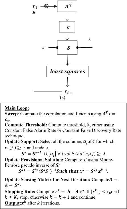
StOMP computes resemblance using inner product of residual vector with the dictionary/basis matrix. Computed coefficients are then thresholded using results from detection theory. Least squares reconstruction is the performed using updated support set. Initialization and other details are given in table 1. Details of StOMP are given in Fig. 2 [20].

Computation of threshold lies at the heart of any IS operator based CS technique. In StOMP threshold is computed as t_k a_k . C7_t is given as ^ = || r j|/ 4m whereas t_k is given as 2 <  t_k <  3 . There value of t_k is empirically adjusted to achieve desirable tradeoff between false discovery and missed discovery. In [20] authors have given detail procedure and analysis about threshold selection.

Table 1. Initialization and parameter settings of StOMP

Task: Approximate the solution of min | x |0 subject to Ax = b

Parameters : w e are given sensing matrix A , the vector b and the error threshold ε 0

Initialization: Program counter k=0, initial solution x ⁰ = 0, initial residue r ⁰= b - A x ⁰= b

And initialize solution support 5 ° = Support{ x ⁰ } = 0

(b)

Fig.2. (a) Block Diagram of StOMP, (b) Main loop of StOMP

• IV.    Simulation Setup

In this study 20 element array is used. Isotropic radiators are assumed. Narrow band assumption is employed. Inter-element spacing of lambda/2 is used.

Another important aspect of simulation is certain subtle differences in both algorithms. These are summarized in table 2.

Table 2. StOMP vs. MUSIC

Property	MUSIC	StOMP
Correlated Sources	Doesn't work/reduced aperture	No issue
Number of Sources	Must be known	Doesn't need the information
Thresholding	NA	Computation of threshold parameter
Spectrum searching for peaks	Yes	No
Spectrum	Continuous	Discrete

Based upon these properties it is somewhat difficult to compare these two algorithms. We would, hence, employ various scenarios for comparison. These are reported in results section.

Error computation is based upon RMSE given by [10];

RMSE =

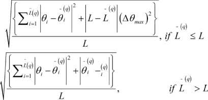
Where;

° = i th source actual location,

~ ⁽ q )

Oi = i source estimated location at q run

~ ⁽ q )                                                            _th

L =Number of estimated sources at qt run L = Actual Number of Sources and

-⁽ q )

O i = arg

{ o min _£ ° , — ° j ) } .

In CS techniques one usually obtains more basis than actually needed. This calls for additional thresholding. Energy based thresholding is applied in this setup. Details are outlined in Fig. 3.

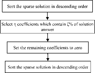
Fig.3. Energy Thresholding

ζ=96 is used in this simulation setup.

• V.    Results

  In first simulation we would randomly generate 2 sources and vary SNR from -5 to 20 dB. We have simulated MUSIC with two variations. In first setup we gave number of sources to MUSIC algorithm, whereas in second we supplied MUSIC with same information that StOMP uses; i.e. we give MUSIC 96% of total sources that can be detected. For 20 element array it works out to be 18 sources. An average of 1000 runs was reported in graphs.

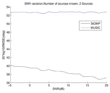
Fig.4. RMSE vs. SNR , 2 sources MUSIC doesn't know sources number

It can be seen that RMSE for MUSIC is much greater than StOMP. Also as SNR increases the error for StOMP decreases whereas it remains almost the same for MUSIC.

In next simulation, reported by Fig. 5, MUSIC is furnished with the knowledge of number of sources. Other parameters remain same. Here we can see that performance of MUSIC improves with SNR. StOMP still performs better than MUSIC.

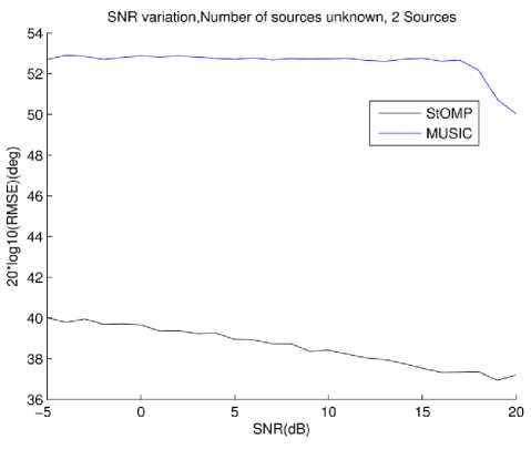
Fig.5. RMSE vs. SNR , 2 sources MUSIC knows sources number

Next algorithms' performance is gauged for greater number of sources. The number of sources is increased to ten Again two variations are simulated. In first, reported by Fig. 6, MUSIC is not supplied with correct knowledge of number of sources and in second, reported by Fig. 7, MUSIC knows number of sources

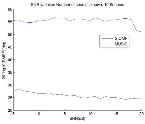
Fig.6. RMSE vs. SNR , 10 sources MUSIC doesn't know sources number

It can be seen that increasing number of sources increases performance of MUSIC degrades a little bit. Another interesting point is improvement of StOMP performance in the same case. This is because number of false discoveries decreases as actual number of sources increases.

In Fig. 7 it is observed that MUSIC performance improves as SNR increases. This is similar to the earlier case of 2 sources.

In both scenarios of Fig. 6 and 7 StOMP outperforms MUSIC. It also remains insensitive to the knowledge of source numbers. RMSE improves with increase in SNR for StOMP in all cases.

We have not simulated the coherent source case as structure of MUSIC breaks down and leads to unstable results.

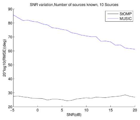
Fig.7. RMSE vs. SNR , 10 sources MUSIC knows sources number

In next simulation we analyze the effect of source separation on RMSE for different SNR levels and sources' numbers. Both scenarios, known and unknown sources' number for MUSIC are simulated and reported.

In first case 2 sources with random location are considered. SNR is kept at 2dB. The separation is varied from 5 degrees to 25 degrees in step of 5 degrees. For each reported point is an average of 1000 simulation runs. The result is reported in Fig. 8. In this case MUSIC doesn't have knowledge of source number.

sepration between sources,Number of Sources unknown, 2 Sources,2 db SNR 54 г

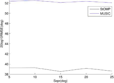
Fig.8. RMSE vs. Source separation 2 sources, 2dB SNR, Source number unknown to MUSIC

The similar scenario in which MUSIC has knowledge of number of sources is reported in Fig. 9.

Again there is slight performance degradation for MUSIC for unknown source number case. However overall the reported graphs are straighter indicating the super resolution capability of both algorithms.

StOMP still outperforms MUSIC in both scenarios. The performance of StOMP again is not dependent on knowledge of source number. Slight oscillation in RMSE for StOMP is due to statistical nature of the algorithm and it hints at imperfect dictionary structure. This is due to symmetrical coherence of bases of steering vector dictionary used in defining the CS setup earlier. Detail proofs of such artifacts are important future research directions.

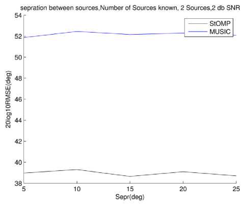
Fig.9. RMSE vs. Source separation 2 sources, 2dB SNR, Source number known to MUSIC

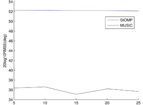
Next simulations are performed with similar parameters as that of Fig. 8 and 9 but SNR is now increased to 20dB.

sepration between sources,Number of Sources unknown, 2 Sources

Sepr(deg)

Fig.10. RMSE vs. Source separation 2 sources, 20dB SNR, Source number unknown to MUSIC

In both Fig. 10 and 11 MUSIC performance improves a little bit when source number is known. StOMP performance is better at both levels of SNR. Also note that SNR improvement does not affect MUSIC whereas it does affect performance of StOMP which improves a higher SNR.

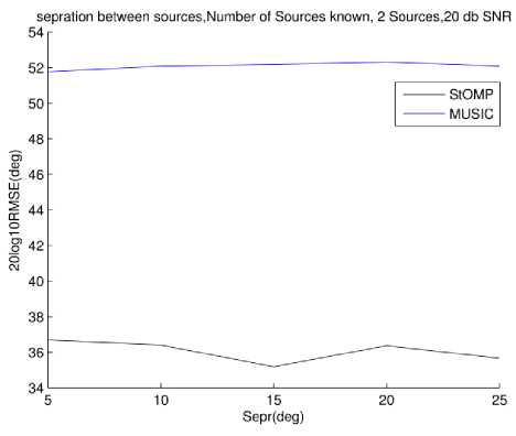
Fig.11. RMSE vs. Source separation 2 sources, 20dB SNR, Source number known to MUSIC

Similar scenarios are reported in Fig. 12 and 15 with number of sources increased to 8.

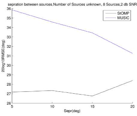
Fig.12. RMSE vs. Source separation 8 sources, 2dB SNR, Source number unknown to MUSIC

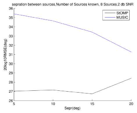
Fig.13. RMSE vs. Source separation 8 sources, 2dB SNR, Source number known to MUSIC

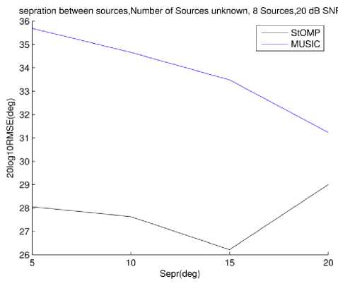
Fig.14. RMSE vs. Source separation 8 sources, 20dB SNR, Source number unknown to MUSIC

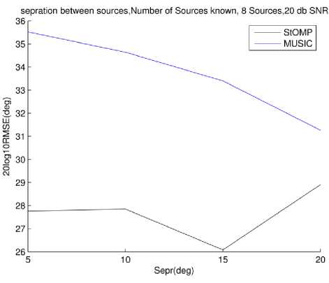
Fig.15. RMSE vs. Source separation 8 sources, 20dB SNR, Source number known to MUSIC

The results reported in Fig. 12 and 15 are quiet similar to the 2 sources case. However the symmetry is more profound now for StOMP. The separation is limited to 20 degrees as it covers the whole spatial extent available. The last case of 25 degree separation could not be simulated but one can extrapolate keeping in mind the symmetry hinted at by 2 sources case.

Finally, effect of number of sensors on DOA estimation performance is reported in Fig. 16 and 19. In these figures we have tested two cases each of low number of sources at low SNR and high number of sources at high SNR. Respective scenarios are reported in figures' caption.

In the cases of Fig. 16 and 17 it can be seen that performance of StOMP algorithm degrades when number of sensors are increased which effectively increases the aperture of the array. This behavior is due to the greedy nature of StOMP algorithm. When array aperture increases so does the total number of bases in the spatial sensing dictionary. This increase in number tends to "confuse" StOMP due to correlated nature of basis. As number of sources is low so chances of selecting a basis near the correct one increases due to larger number of free bases available.

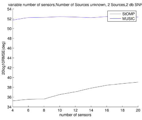
Fig.16. RMSE vs. Number of sensors in array.2 dB, 2 sources. Number of sources unknown to MUSIC

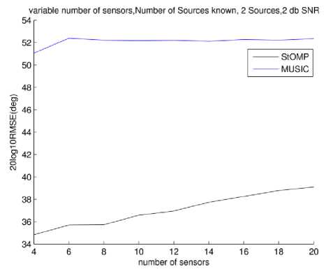
Fig.17. RMSE vs. Number of sensors in array.2 dB, 2 sources. Number of sources unknown to MUSIC

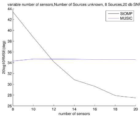
Fig.18. RMSE vs. Number of sensors in array.20 dB, 8 sources. Number of sources unknown to MUSIC

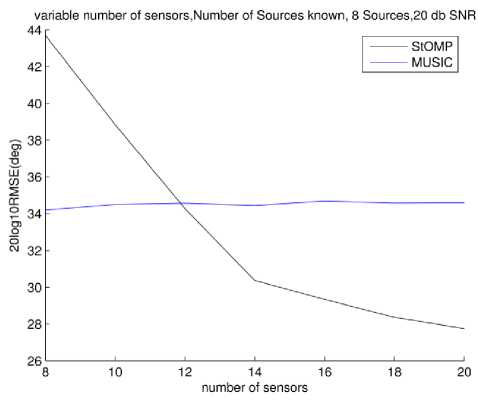
Fig.19. RMSE vs. Number of sensors in array.20 dB, 8 sources. Number of sources known to MUSIC

In Fig. 18 and 19 it is observed that when sensor number is equal to number of sources performance of StOMP degrades. This is because the sparsity assumption no longer holds. When sensor number are relatively larger in proportion to that of sources number the situation improves.

• VI.    Conclusion

The paper presented application of iterative shrinkage operator to the problem of DOA estimation. This application is benchmarked against state of the art MUSIC algorithm.

It is found that StOMP algorithm performs superior in statistical analysis. It has better RMSE for DOA estimation, better resolution of sources and performs comparatively for lesser number of sources.

It is found that MUSIC needs to know the source number and correlated sources can't be handled by MUSIC without reduction in aperture. StOMP not perform superiorly but it is has also none of the restriction MUSIC has.

There is still need to rigorously analyze StOMP for system performance. We need to establish sparsity bounds, recovery probability and particularly need to establish some bound for spatial sensing dictionary. These being the future directions to extend the research presented in this paper.