Level Sets based Directed Surface Extraction

Published Online April 2011 in MECS

The development of rapid prototyping technology makes the demands for medical equipment customized for individual patients increasing [1-4]. A common practice to design such equipment is to use CAD shape data obtained by scanning the individual patient. In this research we focus on such equipment attached to bones as “locking plates” (Fig. 1) or “artificial bones”.

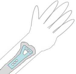
Figure 1. Locking plate.

A shape of the equipment consists of several pieces of surfaces some of which must fit to a surface of a bone of a patient. This surface of a bone can be obtained in the form of a triangular mesh generated from the CT images of the bone with iso-surfacing method such as Marching Cubes [5]. This iso-surface contains the outermost surface of the bone and also complex inner surface of the bone. In our target applications we need only the outermost surface since the equipment is attached to the bone and thus have to extract the outermost surface. As these surfaces generated with the iso-surfacing method are generally closed, it is not so difficult to do so by selecting the largest iso-surface which encloses the other iso-surfaces. However, there are often some holes on the outermost surface of a bone which connects the outermost surface to the inner surface. An example is shown in Fig. 2. The bone always has two surfaces and sometimes the inner surface is connected to the outermost surface (Fig.2 c) by small holes. So we have to remove the inner surface from the desired bone to get the directed outermost surface.

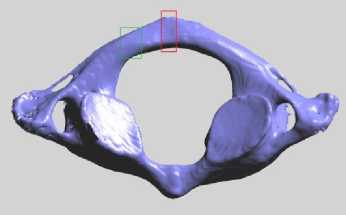
(a). CT model

(b). Sectional view (c). Sectional view

Figure 2. CT model: sectional views of green and red rectangle are given in b and c respectively.

In addition when a bone is articulated to other bones, the outermost surface can be connected to another bone part through a narrow region because of the limited resolution of CT image. We also have to cut the outermost surface at these narrow connections. Moreover, considering the aesthetic reasons, we require the desired bone to be cut off from CT model by optimal cutting plane, which makes the ends of the outermost surface of the desired bone to best represent the shape of the bone. In Fig. 3, suppose two planes (red and green curve) are used to cut a cylindrical model. The plane represented by the green curve is an optimal cutting plane because the cross section is disk and the end of the outermost surface is circling which best represents the shape of the cylindrical model.

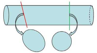
Figure 3. Optimal cutting plane: the green plane makes the cross section best represent the shape of the bone

Once such a directed surface of a bone is got from CT images, it is fed to a reverse engineering system to produce parametric surfaces which are then used to design CAD model of the equipment. To this end, we propose an approach based on level set method to extract such directed outermost surface from CT images. The zero-level set surface is generated at the user interested bone. And then a speed function is used to evolve the surface which fixes part of the zero-level surface to the outermost surface of the interested bone and guarantee the other parts to be optimal cutting plane all the time. In addition, to remove the complex inner surfaces of the bone, a different speed function is used to evolve another zero-level set surface, which is initialized to be a cylindrical surface after considering the shape of bone. Experimentally, with the proposed method, we successfully get the outermost surface from the CT images

• II.    overview

Level set method is a computational technique for tracking a propagating interface over time [6, 7]. The basic idea of level set method is embedding the shape of the objects as the zero level set of a higher dimensional surface. The higher dimensional surface evolves under the influence of the surface features without violating the surface regularity. While the surface evolves, the zero level set contours might develop singularities and sharp corner or they might change topology.

In level set method, a closed surface γ can be expressed in implicit form as γ = { p | φ(p) = 0 }, where φ(p) is timedependent level set function whose absolute value at p is given the distance between p and γ , and its sign depends on whether the point p is inside or outside γ . With forward difference scheme in time, γ can be written in an update form, namely

ф(P,t + 9) = ф(p,t) - |Vф(p,t)| • F(p) • е (1)

where F(p) is the so-called speed function and is bound to be orthogonal to the zero level set and can be arbitrarily defined in order to steer the evolving front propagation toward a desired shape. θ is time interval. For simplicity, in this study 6 = 1, V^(p, t) = 1.

The basic idea of this study is that we generate a zerolevel set surface--cylindrical surface, based on user's specification. It looks like a slice of the bone whose side surface is close to the outermost surface of the bone and the top and bottom surfaces are optimal cutting planes.

With the proposed speed function, the zero-level set surface propagates along the bone without exceeding the outermost surface of the bone. Meanwhile, the top and bottom surfaces are guaranteed to be the optimal cutting plane during its propagation so that whenever zero-level set surface stops moving the ends of the outermost surface can represent the shape of the bone well. Moreover, being optimal cutting planes, the top and bottom surfaces can also be used to detect the narrow connections, for example, by considering the area as they propagate along the bone.

To remove the inner surface of the bone, we can either do it after the zero-level set surface stops moving or during its evolution. Due to the fact that the top and bottom surfaces moves along the bone step by step and the side surface increases slice by slice, we remove the inner during the zero-level set surface evolution since at this moment removing the complex inner surfaces becomes a simple two dimensional problem. Considering the shape of the increased surface in each evolution, we initialize zero-level set surface used to remove the inner surfaces to be a cylindrical surface and then evolve the surface with another speed function which guarantee the surface finally stops at the outermost directed surface and without touching the inner surface. The outermost surface is got by preserving the surface of the bone close to the zero-level set surface.

So in this study two different level set functions with corresponding speed functions are used. To distinguish them, the first zero-level set is named cut level set as it is used to separate the desired bone from the CT model. And the second zero-level set is named removal level set as it is used to remove the inner surface.

Before describing our method in details, we first introduce some basic representations used in the proposed method.

Input to our system is a set of CT images or a volume model V={ p_i } comprised of a series of CT slice images, including a bone in concern. The CT image consists of points (voxels) p i arranged in the 3D grid structure. Each grid point p i is assigned its CT value ρ(p i ). By defining a threshold µ of CT value we can distinguish a foreground (bone) part from the background where ρ( p i )-µ ≥ 0 and ρ( p j )-µ < 0 for the foreground point p i and background point p j respectively. We can also reconstruct a triangular mesh representing the bone surface by using an isosurfacing method named “Dual Contouring” [8] (see Fig. 4). Four triangles are generated around an edge which connects a foreground point p_i and background point p j . Such a foreground point p i is called boundary grid point and each triangle t i of the triangular mesh can be associated with some of these boundary grid points. For clarity we call the mesh Grid-Mesh and the relationship between the boundary grid points and the triangles GridMesh relation . In this paper, B is used to denote the boundary grid points, where В с V and T is used to indicate the generated triangle meshes, where T ={ t i }. In Fig.4 the grid mesh relation is given as g:{t₁,t₂,t₃,t₄}↔ P i e В.

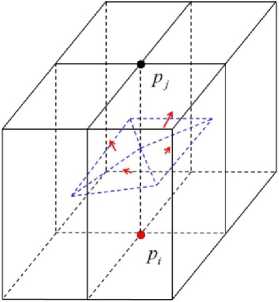
Figure 4. Grid-Mesh relation.

• III.    cut level set evolution

As mentioned above, the proposed method used to cut the desired bone is a kind of “competing front” or “advancing front” method. This kind of methods has been widely used for surface processing, such as [9, 10]. In their methods, they only evolve the meshes of the initialized surface in their normal directions. But in our method, we hope the initialized surface evolves inside the bone. So we keep the side surface of the cylindrical surface close to the outermost surface while the top and bottom surfaces are the optimal cutting plane all the time. Being level set method, the key point of this study is to define a proper speed function so that the zero-level set surface could stop at the desired location.

• A. Initialization

For a different design of equipment, the desired bone is different. Only the designer knows which part is that he wants. So after reconstruction, we request the designer to select a triangle MET from the grid-mesh at the desired bone. And then we get the boundary grid point m E В related to M using the grid-mesh relation, namely g:{M} ^ m E В. The initialization of cut level set is based on finding an optimal cutting plane π* of the bone through m with normal v* and its relevant neighborhood N(π*) .

Relevant neighborhood Let us consider a cutting plane π(q, v) through reference point q with normal v (see Fig. 5). The relevant neighborhood N(π(q, v)) is a group of gird points { p i } which meet the following requirements: (1) p i is boundary grid point; (2) Euclidean distance from p i to π is less than a given threshold δ; (3) p i belongs to the same shape part as q if π encompasses multiple shape parts. Therefore, in Fig. 5, only the blue and green points are the components of N(π(q, v)) . Different colors mean they are on the different side of π(q, v) .

Optimal cutting plane At boundary grid point m, we wish to find an optimal cutting plane π* through m with normal v* which makes the outermost surface of the bone best represent the shape of the bone. Specifically, the normal of π* should be perpendicular to the points’ normal in the relevant neighborhood N(π*). To get the normal v*, we can solve the problem by an iterative approach. For example, we may start from an initial orientation v0 and iteratively update the orientation by solving the following equation:

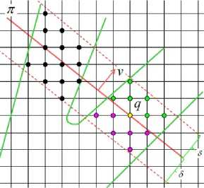
Figure 5. Relevant neighborhood N(π) : blue and green points.

v t+1

argmtn v^£ E R³, Hn^£H = 1

T- pjEN t ^vSn^P j ))

where t > 0, N is the relevant neighborhood for the cutting plane through m with normal v^t at the t-th iteration and n(p j ) is the unit normal at point p j .

This method had been successfully used in Ref. [11] to get the orientation. According to their report, they get the result within 10 iterations for a cylindrical shape model. But for CT model, the result is bad because in most cases CT model is more than a cylindrical model. As a replacement, we solve (2) by a discrete approach. In other words, we first get some candidates { v i } in space and get the optimal one as the orientation v* of π* , which is calculated by the following equation:

v t+1

argmtn v E {v£}, ||v|| = 1

E_Pj EN(v) (v,n(p j ))

where N(v) denotes the relevant neighborhood of optimal cutting plane through m with normal v .

For (3), the result depends on the number of the candidates. Certainly, the more candidates we select, the less chances we miss the exact solution. But we have to spend much time on calculation. To get a proper number of candidates, experiment has been done and shown in Fig. 6. Suppose the optimal cutting plane is through the blue curve. So its normal must be perpendicular to the blue line. Considering the symmetry, the candidates are selected to span 180^ around an end of the blue curve. Comparing the results got with different number of candidates we know 6 candidates bring us the same result as 12 candidates. But it is different for 5 candidates. Thus 6 candidates are enough to get a direction in half space. Therefore, we check 36 candidates in all to get v* in space.

The relevant neighborhood of π* are shown with pink and green points in Fig. 6. Different colors mean they are on the different side of π*. In this study, we suppose all the grid points in N(π*) have the same orientation of their optimal cutting plane in the initialization.

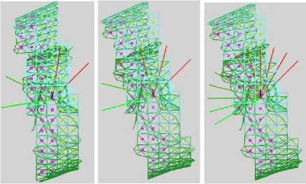
Figure 6. Candidates determination

Because the top surface is also an optimal cutting plane, we evolve the top surface with the following equation:

ot+i = ot + vt5 (4)

where o t+1 denotes the grid point that top surface passes through and v t is the orientation of optimal cutting plane, o 0 =m, v 0 =v*.

With (4), we get a new optimal cutting plane π t+1 through o t+1 with orientation v t . An example is shown in Fig. 7. The green and black points are N ( π t+1 ) and we update the signed distance of those grid points using (1).

To initialize the cut level set surface --- a cylindrical surface, we first give all the grid points signed distance, namely φ(p_i)=d , d>0. After we get N(π*) , we make ф(P j )=-d , Vp j e N(n*) . Please note since we only request the side surface of the cut level set surface to be close to outermost surface, so we don't concern the exact value of d .

With the signed distance, we can generate the zerolevel set surface which looks like the shape shown in Fig. 2(b) and 2(c). Although we talked about the side surface, top and bottom surfaces of the cut level set, these surfaces are not generated during initialization because we only make the signed distance of N(π*) negative. Despite we should change all the grid points inside the outermost surface negative so that we can generate a cylindrical surface, we do not intend to do so because it makes no difference but wasting time for our application. It is not difficult to figure out the surface shown in Fig. 2(b) and 2(c) are the side surfaces and the top and bottom surfaces should pass through the edge of those side surfaces. We will continually use the concepts in the following explanation even though only side surface is generated. The speed function used to evolve the zero level set is introduced in next subsection with which the cut level set will evolve and finally stop at desired location.

B. Speed function

During the evolution, we don't intend to update the signed distance of all the grid points. Alternatively, we just want to update the signed distance of grid points close to the cut level set surface. So how to find the grid points to be updated plays an important role in the evolution. As mentioned above, we wish the cut level set evolves along the bone. So we need the side surface of cut level set to be fixed and the top and bottom surfaces to evolve. As a result, we select the boundary grid points close to cut level set to be updated. With this method, we know grid points close to the side surface of cut level set will not be selected and all the selected grid points are the components of the relevant neighborhood of top and bottom surfaces of the cut level set. Therefore we directly update the relevant neighborhood of top and bottom surfaces. As the top and bottom surfaces are similar. So in the explanation, we take top surface as an example which is in the normal direction.

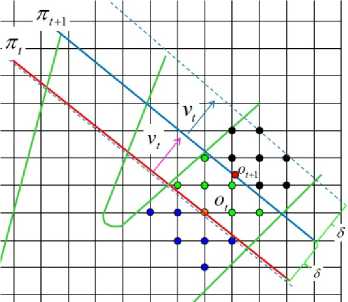
Figure 7. Relevant neighborhood N(π t+1 ): the green and black points

The speed function F(p) is given as follows:

F(p) =

(

KPW _;

dis(p,n _t+1) '   ^t+1

- p) • vt < 0

d; otherwise

where β means the angle between v t and the normal of the

optimal cutting plane through p and dis(p,π t+1 ) means the Euclidean distance from p to π t+1 .

The function f(β) is given as follows:

[  0;P>Pthres

Icos(^) ;otherwise

where β thres is a given threshold.

Generally speaking, the meaning of the speed function is that the closer p is to π t+1 and the smaller β is the larger speed is given. But for the grid points behind π t+1 (the green grid points and o t in Fig. 7) the most important thing is to make sure their signed distance is negative after we update p ^ N(π_t+1) . This can guarantee that no hole is generated on the desired bone.

So far we know π t+1 is parallel to π t as it is got by (4). After we update the signed distance of N(π t+1 ) the top surface of the cut level set moves forward. In Fig. 7, the new top surface may be the blue dash curve and have a different orientation which depends on the signed distance of those black grid points. With (4) we only update the reference anchor of top surface, from o t to o t+1 ; we also need update v t to v t+1 for π t+1 . v t+1 is got by the following equation:

Vt+1^1^ ^(Pj)<0 ^(^(pj)) (7)

P j eN^ t+T )

where n(π(p j )) means the normal of the optimal cutting plane through p j and u is the number of the grid points that φ(p j )<0.

Since we suppose the grid points in a relevant neighborhood have the same orientation of their optimal cutting plane, so we use (7) to get the average normal.

• C. Experimental results

With the proposed procedure, we can evolve cut level set along the bone while making sure the top and bottom surfaces are the optimal cutting planes all the time. Some experimental results are shown in Fig. 8. In the figure, the blue points are those with negative signed distance and the pink and green points indicate the grid points whose signed distance had been updated but still positive. Since the surface is generated based on the grid points with negative signed distance, the occurrence of the pink and green points means to trim the cut level set surface to make the top and bottom surfaces to be optimal cutting planes.

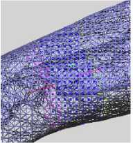
(a) 1 times evolution

(b) 5 times evolution

Figure 8. Front evolution

When the cut level set surface stops moving, we get the related meshes of the gird points with negative signed distance (the blue grid points in Fig. 8) using grid-mesh relation. As a result, only the desired partial bone is got from input images despite the complex inner surfaces are included. In the next section, we will talk about how to remove the complex inner surface with a different level set function.

• III.    Removal level set evolution

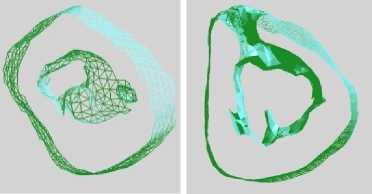
Although the CT model is complicated, the inner surfaces can be divided into two groups according to their connection to the outermost surface, as shown in Fig. 2(b) and 2(c). Those sectional surfaces can be got during cut level set evolution. For example, if we get the related triangles of blue, black or green grid points by grid-mesh relation in Fig. 7, we may get different sectional surface. The basic idea of the proposed removal method is that a cylindrical surface is generated to be the removal level set, which contains a sectional surface. And then the removal level set shrinks under the influence of speed function and finally stops at the outermost surface or the narrow connections if there are. At last, the surface close to the removal level set is kept and other parts are removed.

Before the idea is shown in details, some definitions used in this procedure are given first.

TB : denotes the boundary grid points close to the top and bottom surface of the initialized removal level set surface.

X(p) : is a binary function to indicate the location of the grid point p , Z^o^^^ , ^ is ^the given threshold of the CT value.

T(t,p) : denotes waiting time of a grid point p at time t,

T(t,p) = кв

s.t. p(t,p) = p(t -в,р) = p(t - 2в,р) = - = ^(t - кв,р) ^ p(t - (к + 1)в, p), where 6 is time step.

T_max : denotes the upper limit of the waiting time.

X(t,p) : denotes support ratio for a grid point p ^ B at time t,

n Жр) = n0

where n 1 is the number of the support boundary grid points in a given neighborhood and n 0 is the number of boundary grid points in the given neighborhood ψ.

Please note that all the definitions only used for inner surface removal.

• A.    Initialization

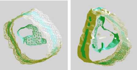
As mentioned above, we initialize the removal level set as a cylindrical surface which contains a sectional surface. Two examples are shown in Fig. 9. The green triangles are the sectional surfaces. The yellow triangles are the initialized removal level sets. In the two examples, the top and bottom surfaces of the removal level set have not been shown except some triangles are shown in Fig. 9(b) to indicate their location. Due to the fact that the bigger the initialized removal level set is, the longer the calculation time will cost, in Fig. 9(b) the removal level set is not an exact cylinder shaped surface at all.

(a) Example 1

(b) Example 2

Figure 9. Removal level set initialization

After we determine the size of the removal level set, signed distance for each grid point is calculated based on the surface. In this study, the grid points inside the removal level set is given a negative signed distance while positive for those outside the removal level set. During the removal level set construction, the Grid-Mesh relation is built at the same time. In addition, the waiting time for all the grid points is zero in initialization, namely т(0,р)=0 , Vp.

• B.    Speed function

We hope the removal level set surface shrinks towards the sectional surface and finally stops at the outermost surface. The shrinking can be done by increase the signed distance φ of each grid point. The speed function is given as follows.

Loop the following procedure for t=0, θ, 2θ, ··· , until the zero level set stops moving.

For each grid point ptB:

If ^(t + 0,p)ф(t,p) > 0, then

F(t,p) = C

Else

F(t,p) = 0

where B indicates the boundary grid points and C is the speed in which zero level set moves towards the sectional surface.

Please note when we talk about the boundary grid point in this subsection, it is only related to the removal level set.

To make certain the removal level set never touches the interior surface; the following speed function is used to update the singed distance of boundary grid points.

For each grid point p £TB:

F(t,p) = 0

T(t + 0, p) = T(t,p)

For each grid point p £ B\TB:

If ^(t,p) >  | , then

x f C,for x(p) = 0 F(t,p) = l0,forzto = 1 T(t + 0, p) = 0

Else

If T(t, p) < ттах then F(t,p) = 0

T(t + 0,p) = t(t,p) + 0

Else

F(f      [C,for X(p) = 1

(t,p)   l0,for z(p) = 0

T(t + 0, p) = 0

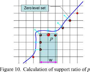
From the proposed speed function we know the most important thing is to calculate the support ratio of a boundary grid point. An example is shown in Fig. 10. Suppose ψ=6 and 3 of neighbors on each side of p . So n₀=6. The candidates are shown as red circle enclosed black. Their orientations are shown in light blue arrows. Only the boundary grid points { q } met the following conditions are the support to p . First, χ(q)=χ(p). Second, n(p)∙n(q)> b and b is a given threshold. In this example, suppose b=0.6 and we know only the boundary grid points on the right side of p are the supports. We get n 1 =1. Thus, we know λ(t,p)=1/6 at this moment. According to the speed function, the level set will cut off part of the feature. In other words, the zero-level set surface will not stop at the current location.

Before calculation, user should define ψ and b according to the model. In Fig. 10, supposing the light blue part is narrow bridge, we hope the level set stop at current location. To this end, we let ψ =4 and b=0.4, then we get λ(t,p)= 3/4. Considering the speed function, we know the zero-level set will stop there as all the boundary grid points had got enough support.

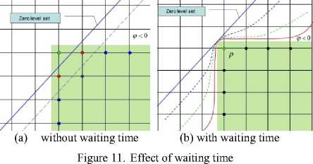
We need the waiting time because the zero-level set surface may arrive at the boundary of the input model at different time. According to the speed function, we know when the zero-level set touches the corner of the model, the support ratio is very low (the green points in Fig. 11(a)). As a result the zero-level set goes into the input model (the blue curve and the dash curve). It is not what we want. After we introduce waiting time to speed function, the evolution is different. As a result the zerolevel set stops at the boundary of the input model (red curve in Fig. 11(b)).

There are several constants to be determined.

Speed C : To keep the stability of level set method, CFL condition that requires the zero level set surface to cross no more than one grid cell each time step must be followed. Thus, we can get the speed by the following equation, namely

C < -e                          (8)

where L is the distance between any two adjacent grid points.

Neighborhood ψ : To calculate the support ratio , we should know the size of the given neighborhood which is determined by the following equation

V =2[ f ]                       (9)

where d is the approximate diameter of the small connections.

Upper limit of waiting time τ max : The calculation of τ max can be done by the following equation:

Т тах = [ ^ ]                    (10)

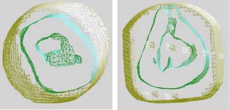
With the proposed speed function, after the removal level set surface stops moving, the results of Fig. 9 are shown in Fig. 12. We can see the removal level set surface (yellow meshes) stops at the outermost surface of the sectional surface. One thing should be noted is since the removal level set surface (yellow meshes) and the sectional surface (green meshes) are generated based on different data set, so they are different even they may share the same related boundary grid points. That is why in Fig. 12(b) some parts of removal level set surface are inside sectional surface while some parts are outside. Although the removal level set surface is different from the sectional surface, it shares the same related boundary grid points with the outermost surface of the sectional surface. So we get the outermost surface based on this fact after the removal level set surface stops moving.

(a) Example 1              (b) Example 2

Figure 12. Final location of removal level set

Outermost surface acquisition We can get the outermost surface using Grid-Mesh relation. The procedure starts from the removal level set surface. We get all the related boundary grid points of the removal level set surface and find and preserve the related meshes on the sectional surface which constitute the outermost surface that we want. The results of Fig. 12 are shown in Fig. 13.

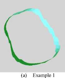
Figure 13. Directed sectional surface

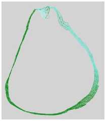
(b) Example 2

• IV.    Experimental results

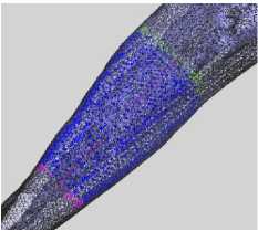
After using the method proposed in this paper, we get some experimental results and show them in Fig. 14. The directed surfaces are shown in green in Fig. 14(a) and light blue in Fig. 14(c). The extracted directed surfaces are shown in Fig. 14(b) and Fig. 14(d) respectively. It is obvious that the proposed method can be used to extract the directed outermost surface from CT images.

• V.    Discussion

In this paper we propose an approach based on level set method to extract the outermost surface of a desired partial bone form CT images. A level set function with a novel speed function is used to cut the desired bone from the CT images. In this procedure, making sure the ends of the bone are the optimal cutting plane is the most important thing. When a sectional surface including complex inner surface is got, another level set function with a different speed function is used to remove the inner surface. Experimentally, the proposed method succeeds extracting the outermost surface from CT images.

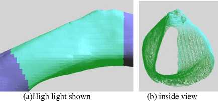
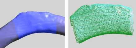
(c) High light shown (d) Outermost surface

Figure 14. Experimental results

This method offers many opportunities for improvements and modifications. For the inner surface removal, in most cases the removal level set shares the same related boundary grid points with the outermost surface. But for a high concave surface, it may be different. So a new way to utilize the removal level set surface should be introduced to make the approach more robust. In addition, although the outermost surface is extracted from the CT images, the edge of the surface is rough. For design, a smoothing method should be introduced to smooth the edge. Moreover, so far we have no experimental results to show the proposed method being used to detect the narrow connections. In the future, we will try out the method on some other models.