Low-energy Earth – Moon – Earth flight trajectory design using optimization procedures

Introduction. The preparation of lunar expeditions is currently one of the key objectives in the space industry [1; 2]. Depending on the mission aims, one of three programs is typically implemented: a lunar landing, lunar orbit reaching, or a lunar flyby. In the last mission type, when the spacecraft must return to the Earth, it is necessary to determine the trajectory parameters that ensure the spacecraft arrival at the Earth upper atmosphereу layer during the flight terminal phase.

There are different approaches to spacecraft trajectory design. The method proposed in [3] involves analytical computation of trajectory points combined with numerical integration of the spacecraft equations of motion. The resulting flight profile assumes the three-impulse correction maneuvers. In [4], the trajectory is constructed based on a spacecraft dynamical model using precomputed ephemerides of the Earth, Moon, and Sun. To obtain a continuous flight trajectory, an iterative adjustment of the motion parameters is applied.

In existing methods, the solution to this problem is typically obtained by solving a boundary value problem through numerical integration of differential equations describing the spacecraft dynamics under the gravitational influence of celestial bodies. However, due to the large number of parameters involved, the computational cost and time required to obtain a solution by such methods are too high. Therefore, in this study, it is proposed to construct the spacecraft flight trajectory using a combination of an analytical approach and a numerical optimization method. The proposed approach to solve the problem of interest includes procedure of the orbital parameters and the spacecraft state vector computation, as well as the optimization procedure, that is schematically shown in Figure 1.

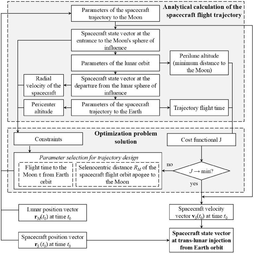
Рис. 1. Схема вычислений в предлагаемом подходе к формированию траектории полёта КА

Fig. 1. Calculation scheme in the proposed approach to forming the flight trajectory of a spacecraft

In the general case, such optimization problem is multi-extremal; therefore, it is reasonable to apply evolutionary optimization methods, particularly the genetic algorithm, as a numerical method [5]. The genetic algorithm is widely used in solving optimization problems in the aerospace [6], for example, for tuning control loops of unmanned aerial vehicle (UAV) systems [7], configuring spacecraft stabilization systems during reaction wheel spin-up [8], tuning control systems of dual-rotor aerodynamic platforms [9], and designing pitch programs for launch vehicle reaching the desired orbit [10].

Spacecraft flight profile design.

The design of spacecraft flight profile is performed using the spheres of influence method (see Fig. 2). First, the geocentric flight trajectory to the Moon is determined, ensuring the spacecraft transfer from Earth sphere of influence to the one of the Moon. Then, the flight trajectory of the spacecraft around the Moon within the lunar sphere of influence is computed. At the final stage, the flight trajectory of the spacecraft departures from the Moon is determined. To guarantee the spacecraft return to the Earth orbit and to achieve the required altitude of the perigee of the desired orbit, an impulse correction is necessary [11; 12].

To reduce the energy of the Earth–Moon–Earth flight, a passive flight is considered, where a single velocity impulse is performed at the Earth orbit after the launch phase is completed. Consequently, the parameters of each segment of the spacecraft flight trajectory, including one from the Moon back to the Earth, depend only on the initial conditions.

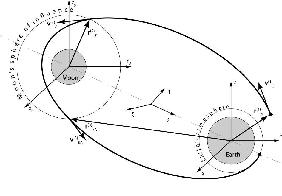
Рис. 2. Схема полёта КА

Fig. 2. Flight diagram of the spacecraft

The Earth–Moon–Earth flight trajectory is divided into three segments, the orbits of each are represented as conic sections [13]. The first segment of the flight trajectory represents the geocentric orbit of the spacecraft flight to the Moon. In the second segment, the trajectory corresponds to the spacecraft flight within the Moon sphere of influence along a selenocentric orbit. The final, third segment represents the spacecraft departure from the Moon orbit and its return to the Earth along a geocentric orbit. Further in the notation, for example in r _S ⁽¹⁾ , the superscript indicates the parameter association with the k -th orbit (segment), where k = 1,2,3.

Let’s consider the first segment of the Earth–Moon–Earth flight. It is defined by the geocentric radius vector of the spacecraft r _S ⁽¹⁾ at the specified launch point, the radius vector of the apogee of the first orbit r ¹ and the time of flight to apogee T _{1 - r} (see Figure 3). The orbit apogee is located on the extension of the line segment connecting the Earth and the Moon centers of masses at the predicted point:

(1)                            MC 0-----1-1 ) P ra     rM(t0 + С1-Г) +11    ,           \ll RM ’                                          (1)

^r M ⁽ t 0 + ^T 1 - 1 ‘ )

where 1 0 is the spacecraft launch time, s; r _M ( 1 0 + T _{1 - r} ) is the geocentric radius vector of the Moon at time 1 0 + T _{1 - r} , km; R_M is the selenocentric distance to the apogee of the first orbit, km.

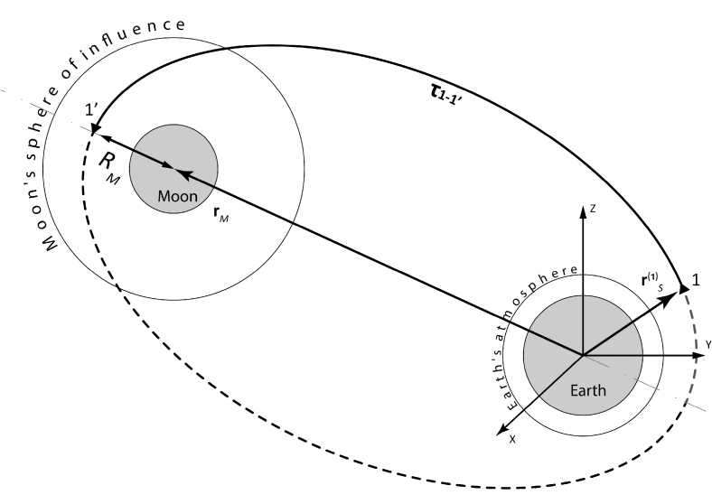
Рис. 3. Формирование орбиты полёта КА от Земли к Луне

Fig. 3. Formation of the orbit of the spacecraft flight from the Earth to the Moon

Based on the calculated rP , r ^ ¹ ) and T _{1 - r} values the elements of the first flight orbit are then determined as follows

{ e", p", ^c 1 0 ), n '¹' ,»" ) , i" } = f ( г ; ", c t , - , . ) ,                        (2)

where e is the eccentricity; p is the focal parameter, km; Э ( 1 ₀ ) is the spacecraft true anomaly at the launch moment 1 ₀ , degrees; П is the right ascension, degrees; o is the argument of pericenter, degrees; i is the inclination, degrees; f ( • ) is denoted the procedure used to compute all these parameters, a detailed description of which is given in [10]. Further, the true anomaly 3 ⁽¹⁾(^) of the spacecraft and the geocentric radius vector to the Moon r _M ( t ₁ ) at the time t ₁ when the spacecraft reaches the entry point into its sphere of influence are calculated.

Let’s consider the second segment of the Earth–Moon–Earth flight. To begin with, the selenocentric radius vector of the spacecraft r _S ⁽²⁾ and the spacecraft velocity vector v ⁽ _S ²⁾ are determined as follows:

{< • v? } = f ( Г м ( t , ), e "’, p "', ^’с t , ), П" ) ,^", i‘" ) ,                      (3)

Based on the calculated r _S ⁽²⁾ and v ⁽ _S ²⁾ , the parameters of the second flight segment that are the selenocentric orbit of the spacecraft within the Moon sphere of influence are determined as follows:

{ e ®, p '=’, 9^m( t ,), fl^, o®, i ^m, r ^’ } = f ( r® , v® ) ,                      (4)

where r _n ⁽²⁾ is the pericenter radius of the orbit, km. Then the true anomaly 3 ⁽²⁾( 1 ₂) of the spacecraft and the geocentric radius vector of the Moon r _M ( t ₂ ) at the time t ₂ at the spacecraft leaving point from the Moon’s sphere of influence are determined.

Let’s consider the third segment of the Earth–Moon–Earth flight. First, the geocentric radius vector of the spacecraft r _S ⁽³⁾ and the spacecraft velocity vector v ⁽ _S ³⁾ are calculated as follows:

{r<3), v} = f (e<”, p(2), Э<”(12), tf),»'”, i<”),(5)

Based on the obtained values, the parameters of the third flight segment that are parameters of the geocentric orbit of the spacecraft from the Moon to Earth, are determined as follows:

{e , p<3', »<3'( I,), й«, .   i , r®, f( 12), t,( = f (rЛ vS").(6)

where v _r ( t ₂ ) is the radial velocity of the spacecraft at the spacecraft leaving point from the Moon sphere of influence, km/s; t ₃ – the time of reaching the perigee of the third orbit, s.

After that, the total flight time is determined according to the following expression tflight = t3 - t0 •

Trajectory Design Using Optimization Procedures. Each spacecraft orbit is characterized by a set of Keplerian elements. Since the spacecraft flight is affected by a single correction impulse at the beginning of the flight, the flight trajectory of the second and third segments is determined by the parameters of the first orbit. Given the known launch point of the spacecraft, design the first orbit requires to specify the selenocentric distance R M to the orbit apogee and the spacecraft flight time T _{1 - r} to that point. Consequently, the vector of initial values is defined as follows:

xo =

R M

Tn'

Thus, for the considered problem of the flight trajectory design, the optimization problem can be formulated, which aims to select such initial conditions that minimize the closest distance spacecraft approaches to the Moon and the total flight time along that trajectory, i.e.,

J = ^a₁ w 1 ( r² ) +a ₂ w ₂ A t ² ^min ,

where r^ is the distance of the closest spacecraft approach to the Moon, km; a i are the normalization coefficients; w_i are the weighting coefficients.

For the selected initial parameters, the upper ( R max , T _{1 - 1max}) and lower ( R min , T _{1 - r} mn ) bounds define the feasible parameters region are formulated as follows:

^R min

s R л s R mx

^1 1'     — ^1 1' — ^1 1'

1-1 min      1-1       1-1 max

Additionally, the nonlinear constraints are included in the optimization problem. They allow us to consider the spacecraft entry point into the Moon sphere of influence and the direction of the spacecraft at the point of leaving this sphere that is determined by the radial velocity sign and the spacecraft arrival to the Earth atmosphere upper layer. These conditions can be written as follows:

fv- S0

■ r“ - (R + ham ) S 0

||r ( t 1 ) - Г м ( t 1 )|| - R in^e S 0

where v_r ⁽³⁾ is the radial velocity of the spacecraft at the leaving point from the Moon’s sphere of influ-

ence, km/s; r _π ⁽³⁾ is the perigee radius of the third orbit, km; R_E is the Earth equatorial radius, km; h_atm is the atmosphere upper layer height, km; r _S ( t ₁ ) , r _M ( t ₁ ) is the geocentric radius vectors of the spacecraft and the Moon at the time t ₁ of entry point into the Moon’s sphere of influence of radius R_influence , km.

A genetic algorithm is used to solve the optimization problem. The chromosome consists of the selenocentric distance R_M to the apocenter of the first orbit and the spacecraft flight time τ _{1 - 1 ′} to that point from Earth launch orbit. A vector composed of these quantities forms an individual. A set of individuals constitutes a population that evolves at each iteration of the genetic algorithm. Figure 4 shows the solution space of the functional (9) under constraints (10) and (11). It is evident that the solution to the optimization problem is highly nonlinear.

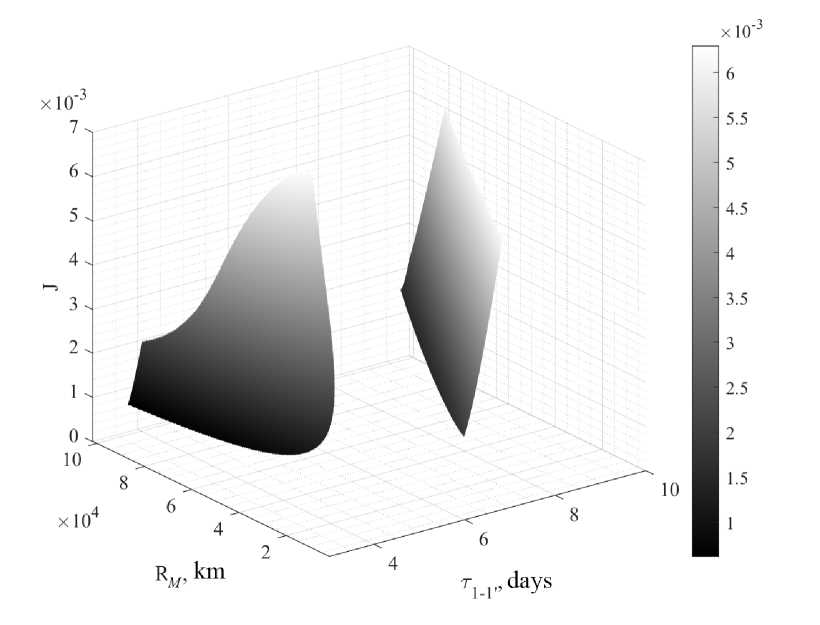
Рис. 4. Пространство решений задачи оптимизации

Fig. 4. Solution space of the optimization problem

Results of the Earth–Moon–Earth Flight Trajectory Parameter Calculation

To assess the correctness of the flight trajectory design, numerical integration of the differential equations describing the spacecraft motion under the gravitational influence of the Earth, Moon, and Sun is performed. The mathematical model of the spacecraft is based on the Newton second law, which defines as follows:

N

F = -Gm M rS ri S        S ∑i i i rS - ri j

where FS is the total force acting on the spacecraft, kg∙km/s²; mS is the spacecraft mass, kg; Mi is the mass of the i‑th body of the Solar System, kg; rS is the spacecraft radius vector, km; ri is the radius vector defining the position of the i‑th body of the Solar System, km; G is the gravitational constant, km³/(kg∙s²). For numerical simulation, the system is converted to the standard Cauchy form.

Table 1 lists the parameters R M and T _{1 - r} computed via proposed optimization problem, along with the orbital elements and state vectors of the spacecraft and the Moon at the launch time t ₀ . The initial population size of individuals in the genetic algorithm was set to 500.

Table 1

Flight trajectory parameters

Parameter	Value
Selenocentric distance RM to the apogee of the first orbit, km	60852.67531856347
Flight time T 1 - r to the apogee of the first orbit, s	497861.4404235960
Elements of the first orbit: (1) eccentricity e focal parameter p (1) , km right ascension Q (1), degrees argument of pericenter Ю (1), degrees (1) inclination i , degrees spacecraft true anomaly 9 ( 1 0 ) at the launch moment 1 0 , degrees spacecraft true anomaly 9 (') ( t 1 ) at the time t 1 of entry into the Moon’s sphere of influence, degrees	0.970233718560075 12946.40576465826 7.801256161798105 27.963990027519067 27.517114189458532 0 178.7634087547173
Elements of the second orbit: (2) eccentricity e (2) focal parameter p , km right ascension Q ( 2) , degrees (2) argument of pericenter Ю , degrees (2) inclination i , degrees spacecraft true anomaly 9 (2) ( t 1 ) at the time t 1 of entry into the Moon’s sphere of influence, degrees spacecraft true anomaly Э (2 ) ( 1 2 ) at the time 1 2 of exit from the Moon’s sphere of influence, degrees	8.337589049815842 550659.8331189135 187.8012561617982 329.9971957197925 152.4828858105415 –25.971322612494077 25.971322612494077
Elements of the third orbit: (3) eccentricity e (3) focal parameter p , km right ascension Q (3), degrees (3) argument of pericenter Ю , degrees inclination i (3) , degrees spacecraft true anomaly 3 (3) ( 1 2 ) at the time 1 2 of exit from the Moon’s sphere of influence, degrees	0.971190044826021 12558.44980487381 7.801256161798059 26.575852741837750 27.517114189458436 181.5293711525792
Geocentric radius vector of the spacecraft r КА ( t 0 ) at the launch point, km		’ 5379,14523655473 ’ 3495,17652028344 _ 1423,57950818001 _
Spacecraft velocity vector v КА ( t 0 ) at the launch point, km/s		Г- 6.24160075029378 7.78883694322032 4.46137142580742	J

Table 1 (continued)

Parameter	Value
Geocentric radius vector of the Moon r Л ( t 0 ) at the launch point, km		~- 312078,982157000 ~ 213237,985181000 132125,221950000
Velocity vector of the Moon v Л ( t 0 ) at the launch point, km/s		Г- 0,581440000000000 - 0,707535000000000 - 0,324062000000000	1 1

Fig. 5–6 show the spacecraft flight trajectory, including curves in the shape of conic sections. The parameters of this trajectory were selected using the procedure described via the genetic algorithm. Additionally, the trajectory obtained through numerical integration of the differential equations using the same initial conditions is also shown. The plots demonstrate that each flight trajectory ensures the spacecraft flyby of the Moon and its return to Earth atmosphere.

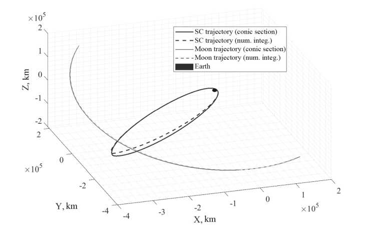
Рис. 5. Траектория перелёта КА в экваториальной системе координат

• Fig. 5. Spacecraft flight trajectory in the equatorial coordinate system

The results presented in this study show the effectiveness of using the spheres of influence method in combination with optimization procedures for designing the Earth – Moon – Earth type flight trajectories. The designed spacecraft flight profile demonstrates that a single velocity impulse at the Earth orbit is the energy-efficient solution, including both the flyby of the Moon and the spacecraft return of the Earth orbit.

The use of the genetic algorithm to solve the optimization problem made it possible to minimize both the spacecraft distance of the closest spacecraft approach to the Moon and the total flight time. This demonstrates the applicability of using evolutionary optimization methods for celestial mechanics problems, that are characterized by strong nonlinearity and the presence of multiple local extrema [14].

A comparative analysis showed that the obtained flight trajectory using the conic section method and through numerical integration of the equations of motion almost coincide. This result confirms the correctness of the proposed flight trajectory design methodology and demonstrates its applicability for preliminary mission design. The results can be used in the preliminary design of missions like the Apollo programs (NASA) or modern return mission projects under the Artemis initiative [15].

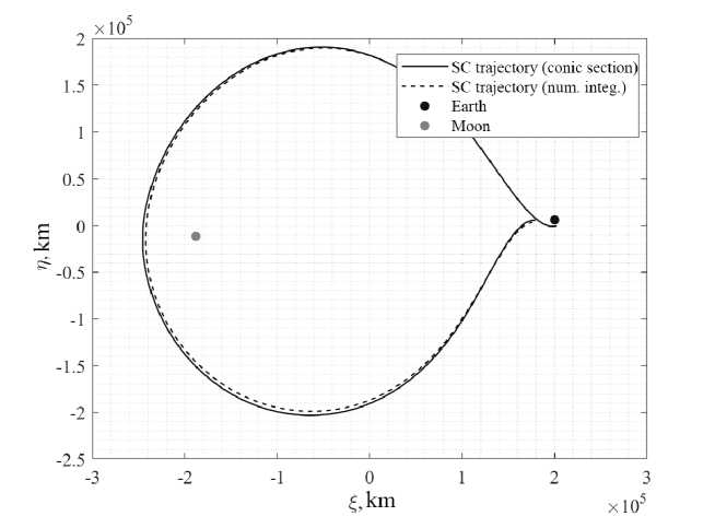
Рис. 6. Траектория перелёта КА в барицентрической системе координат

Fig. 6. Spacecraft flight trajectory in the barycentric coordinate system

Conclusion. In this study, a low-energy the Earth–Moon–Earth flight trajectory was calculated using a combination of the spheres of influence method and the genetic algorithm. The flight trajectory was divided into three segments, each represented as an orbit in the form of a conic section. The shape of the entire trajectory is determined by the initial conditions; therefore, to ensure a lunar flyby and return to Earth orbit, high accuracy of the initial conditions is required.

To construct the spacecraft flight profile, an optimization problem was formulated and numerically solved using a genetic algorithm. The parameters required to form the spacecraft flight orbit to the Moon from the Earth orbit were selected. The optimization problem aimed to minimize both the spacecraft distance of the closest spacecraft approach to the Moon and the flight time along that trajectory, under constraints on the spacecraft entry into the Moon’s sphere of influence and the condition determining its direction of motion. That eventually ensured a successful lunar flyby and return to Earth orbit.

It was found that varying the weighting coefficients in the fitness function in the genetic algorithm allows for the generation different spacecraft flight trajectories, including a lunar gravity-assist maneuver for flights to other celestial bodies. Thus, it can be concluded that using an optimization problem with the genetic algorithm as a numerical solver provides us with a more efficient calculation of spacecraft flight trajectories in lunar missions.