Machine Learning and Software Quality Prediction: As an Expert System

Автор: Ekbal A. Rashid, Srikanta B. Patnaik, Vandana C. Bhattacherjee

Журнал: International Journal of Information Engineering and Electronic Business(IJIEEB) @ijieeb

Статья в выпуске: 2 vol.6, 2014 года.

Бесплатный доступ

To improve the software quality the number of errors from the software must be removed. The research paper presents a study towards machine learning and software quality prediction as an expert system. The purpose of this paper is to apply the machine learning approaches, such as case-based reasoning, to predict software quality. The main objective of this research is to minimize software costs. Predict the error in software module correctly and use the results in future estimation. The novel idea behind this system is that Knowledge base (KBS) building is an important task in CBR and the knowledge base can be built based on world new problems along with world new solutions. Second, reducing the maintenance cost by removing the duplicate record set from the KBS. Third, error prediction with the help of similarity functions. In this research four similarity functions have been used and these are Euclidean, Manhattan, Canberra, and Exponential. We feel that case-based models are particularly useful when it is difficult to define actual rules about a problem domain. For this purpose we have developed a case-based reasoning model and have validated it upon student data. It was observed that, Euclidean and Exponential both are good for error calculation in comparison to Manhattan and Canberra after performing five experiments. In order to obtain a result we have used indigenous tool. For finding the mean and standard deviation, SPSS version 16 and for generating graphs MATLAB 7.10.0 version have been used as an analyzing tool.

Еще

Machine Learning, Software Quality prediction, Case-Based Reasoning, Knowledge base building, Distance functions, Expert System

Короткий адрес: https://sciup.org/15013241

IDR: 15013241

Текст научной статьи Machine Learning and Software Quality Prediction: As an Expert System

Published Online April 2014 in MECS

Due to Lack of sufficient tools to evaluate and predict software quality is one of the major challenges in software engineering field. Identifying and locating faults in software projects is a hard work. Particularly, when project sizes grow, this task becomes costly with complicated testing and evaluation mechanisms. On the other hand, measuring software in a continuous and disciplined manner brings many advantages such as accurate estimation of maintenance costs and schedules, and enhancing process and product qualities. Thorough study of software metric data also gives important clues about the position of possible faults in a module. The aim of this research is to establish a technique for identifying software faults using machine learning methods. It is very common to see large projects being undertaken now a day. The software being developed in such projects goes through many phases of development and can be very complicated in terms of quality assessment. There will always be a concern for proper quality and effective cost estimation of such software. This can be rather tricky as the project being a large one may cover several unknown and unseen factors that might previously be very difficult to judge. Software fault prediction poses great challenges because fault data may not be available for the entire software module in the training data. In such cases machine learning technique like case-based reasoning (CBR) can be successfully applied to fault diagnosis for customer service support. CBR systems use nearest neighbor algorithm for retrieval of cases from the Knowledge base. Other machine learning techniques have also been extensively used for software quality (fault) prediction. The majority of today's software quality estimation models are built on using data from projects of a particular organization. Using such data has well known benefits such as ease of understanding and controlling of collecting data [3]. But different researchers have reported contradictory results using different software quality estimation modeling techniques. It is still difficult to generalize many of the obtain results. This is due to the characteristics of the datasets being used and dataset’s small size. Correct prediction of the software fault or maintain a software system is one of the most serious activities in managing software project. Software reliability provides measurement of software dependability in which probability of failure is generally time dependent. Various software quality characteristics have been suggested by authors such as James McCall and Barry Boehm. There have been differences in opinion regarding the exact definitions of the qualities of good software. For example maintainability has been used to define the ease with which an error can be located and rectified in the software. This definition also includes the ease with which changes can be incorporated in the software [4].

The rest of the paper is structured as follows: Section II gives the background and related work, Section III discussed learning methods in brief, Section IV describe learning/prediction system, Section V describes software quality in brief, Section VI discussed about distance functions, Section VII describes the methodology, Section VIII discussed Proposed model. In Section IX we discussed estimation criteria; Section X describes the research category. Experimental analysis and result has been presented in Section XI. A conclusion has been presented in Section XII and Section XIII ends the paper with concluding future scope. The appendix provides the detail information about results of five experiments in a tabular form (see table 1 to table 5) along with graphs.

II. Background and related work

In the context of software fault prediction, most research works have focused on fault modules. The difficulty of software fault and maintainability is an important part of software project development. Software size and software fault data have regularly been used in the development of models that predict software quality. A few software quality models predict the quality of software modules as also faulty or non faulty [20], [21]. Nowadays one of the major application areas for case-based reasoning (CBR) in the field of health sciences, multiagent systems as well as in Web-based planning. Research on CBR in the area is growing, but most of the systems are still prototypes and not available in the market as commercial products. However, many of the systems are intended to be commercialized [22]. There is a little, but increasing piece of work in which machine learning method is used in the software quality (fault) prediction task. Recent age is more worried about the quality of software. Wide research is being carried out in this direction. The main thrust in modern software engineering research is centered on trying to build tools that can enhance software quality. Many researchers have used AI-Based approach like Case-Based Reasoning (CBR), Genetic Algorithm (GA), Neural Network (NN), etc. Khan et al. [7] mentioned that, when software quality was predicted, the main objective was to predict reliability and stability of the software. Becker et al. [8] was predicted performance of the software. Current software fault prediction models frequently involve using supervised learning methods to train a software fault prediction model. Predicting the quality of the software product during its development phase is a challenging job especially when software sizes grow. Zhong et. al has used unsupervised Learning techniques to build a software quality estimation system [5]. Case-based reasoning has also been used by Kadoda et. al in [1]. Myrtveit et al in [2] and Ganesan et. al in [3] have also studied CBR was applied to software quality modeling of a family of complete industrial software systems and the accuracy is measured better than a corresponding multiple linear regression model in predicting the number of design faults. Aamodt and Plaza are given the case-based reasoning cycle [10]. Rashid et. al emphasized on the importance of software quality prediction and accuracy of case-based estimation model [6] [9].

III. Learning/prediction system

Learning or training methods can be broadly classified into three basic types [19].

• Supervised Learning: When the actual response varies from target response then network generates an error signal. To minimize the error we need a supervisor or teacher, hence the name supervised learning.
• Unsupervised Learning: Unsupervised learning does not require a supervisor or teacher, it needs certain guidelines to make groups. Grouping can be done on the basis of the pattern or property of the object.
• Reinforcement learning: It is similar to supervised learning. Through this method the teacher does not mention how nearer is the actual output to the desired output. Therefore error generated during reinforced learning is binary.

Machine learning techniques have the capability to predict software quality in the early stages of software development. Some of them can be applied if previous data (Training data) is available in the knowledge base. In this research work we have used case-based reasoning (CBR) as a machine learning technique. The interactive learning / prediction system can be seen in figure 1. A user can access the prediction system using the given interface to learn new problems and get the predicted outputs (see figure1). The components of the prediction system are as follows:

1) Interface: It is the point of interaction.
2) Estimation/ Prediction system: Estimating or

predicting a system is typically done by learning from the previous experience and provides knowledge for future solutions to some extent.

3) Machine learning algorithm: Case-based reasoning has been used as a machine learning algorithm where the method of solving a new case(s) based on the solutions on similar previous cases.
4) Training data: The training data used in this research work are collected from the students of computer science and engineering from the university campus,

written in high-level language (C++), They are maintained by faculty, supported by the laboratory staffs, resources like computers, software etc.

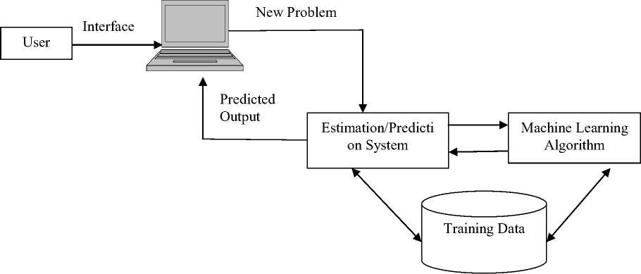
Fig 1: Interactive learning/prediction System

IV. Software quality

Since quality is the first step for improvement in anything, to achieve an improved state of affairs, quality must be precisely defined and appropriately measured. But very often in quality engineering and management, the term quality is misunderstood on account of its ambiguous characteristics. The ambiguity aspect of quality owes its origin from the following [17];

1. Quality being multi-dimensional with dimensions of entity of interest, the viewpoint on that entity and the quality attributes of that entity gets interpreted differently depending upon the situation and interpreter.
2. On the basis of conceptualizing quality, it may be referred either in its broadest sense or in its precise connotation.
3. Being an element of our every day language, quality may be interpreted differently depending upon the uses – popular or professional.

However as the focus of this research will be around the quality of software which is a sort of the professional use of the concept quality as against the popular use of the same, the third point mentioned above duly makes it very clear how quality in popular view is quite different from quality in professional view and hence it draws our attention to take care.

V. Selection of distance functions

Many literatures are reviewed on case-based reasoning and neural network [11] [12] [13]. A similarity function determines, for a given case, the most similar cases from the knowledge base (i.e. Training data). The function computes the distance between the new case and every other case in the knowledge base. In this study four types of similarity functions are considered and they include the Euclidean distance, Canberra distance, Exponential distance and the Manhattan distance.

Suppose a record set S1 of n fields has following values u1, u2,…, un for the n fields respectively. Similarly a record set S2 of the same type with field values v1, v2, …, vn. Table 1 shows the definitions of four distance functions which is used in our analysis.

Table 1: Distance functions

Distance dist (S1, S2) with equal weights of all attributes

1) Euclidean distance ( dist e )

n

diste(S1,S2) = У (w,(u, -v,))2

_______________L±1______________(111

2) Manhattan distance (dist_m)

distm(S1,S2) = £w,.|u,-Vi | i=1(2.1)

3) Canberra distance (dist c )

distc (S1 S2) = У w, I u, - v, I/ I u, + v, I

_______________________________________________(3.1)

4) Exponential distance (dist_ex)

distex (S1, S 2) = £ w,( ed )

^, = 1 (4.1)

Where d= (U^-~viY

A. Euclidean Distance Function:

The most popular dissimilarity measure or distance is the Euclidean distance. Accepts the record set as input and finds the matching cases from the knowledge base. This similarity function is probably the most commonly used distance measures of dissimilarity between feature vectors [6]. The distance is calculated by taking the weighted distance between the new case and an existing case. The weight associated with each independent variable is provided by the user during run time. This distance is also commonly used when the record set contains quantitative attributes, which is given below:

The Weighted Euclidian distance (WED) of S1 from S2 is:

dist ( S 1, S 2)

Е (wi(. ui - vi))2

i = 1

B. Manhattan Distance Function:

This similarity function is sometimes called the city block distance or absolute distance or taxicab distance [6]. It is computed by taking the weighted sum of absolute value of the difference in independent variables between the new case and an existing case. The weight associated with each independent variable is provided by the user during run time.

The Weighted Manhattan distance (WMD) of S1 from S2 is:

distm (S 1, S 2) = E wi I ui - vi I i=1

C. Canberra Distance Function:

The Canberra distance was introduced in the year 1966 and refined in 1967 by G. N. Lance and W. T. Williams [15] [16]. It is a numerical measure of the distance between two pairs of points in a vector space. The weight associated with each independent variable is provided by the user during run time.

The Weighted Canberra distance (WCD) of S1 from S2 is:

distc (S 1, S2) = Е wi 1 ui - vi И ui + vi 1 i=1

D. Exponential Distance Function:

The Exponential distance function is a mathematical function expd (e, d) where d is a variable and e is the constant which is equal to approximately 2. 71828 [14]. The weight associated with independent variable is provided by the user during run time. The distance is calculated by taking the weighted distance between the new case and an existing case.

The Weighted Exponential distance (WEXD) of S1 from S2 is:

diStex (S 1, S2) = Е wi (ed ) Where d= N (ui - vi )2

i = 1

VI. Methodology

We observe software quality (fault) as a multi-dimensional idea, consisting of such properties of the software as maintainability, correctness, flexibility, error proneness, changeability etc. The training data used in this paper are collected from the students of computer science and engineering from the university campus, written in high-level language (C++), They are maintained by faculty, supported by the laboratory staffs, resources like computers, software etc. For each program we have evaluated the students five times.

In this study data collected from students included the following metrics:

• Size metrics (LOC)
• Code documentation metrics (comment lines, blank lines)
• Number of functions or procedures.
• Difficulty level of Software.
• Experience of Programmer in Year
• Development Time
• Number of Variables

The values for lines of code, number of functions, level of difficulty, experience, development time and a number of variables were collected from programs developed by students of the university campus over a period of 1 year.

VII. Proposed model

The parameters selected for the model were based upon the following assumptions.

• The time constraint or development time affects the quality level.
• The mental discrimination required to design and code a program depends upon the numbers of functions and number of variable
• The number of functions is a predictor of how much effort is required to develop a program.
• The programming language exposure / experience of a programmer affect the quality level.
• The inherent program difficulty level also affects the quality level.

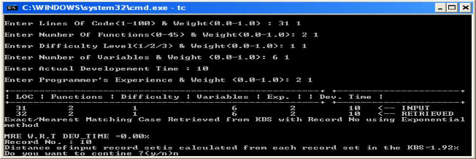
Through this model (see figure 2) user can take input of different attributes of software (the attributes of software used LOC, NOF, DL, NOV, DT, PEX as a threshold vector)

and get output as a exact/nearest matching case from the knowledge base (KBS). In this paper first, we have built a KBS. Second, we have given the emphasis on how to reduce the maintenance cost. For reducing the maintenance cost we are removing the duplicate record set from the KBS. Third, the magnitude of relative error is calculated with the help of distance functions. It can be seen as a snapshot (see snapshot 1 through 7). Therefore one can identify the distance functions which are more efficient for error prediction. Details information regarding separate experiment results can be seen in the tabular form (See appendix).

A. Input Data Module

This module accepts the values of various parameters from the user. It also has the provision of assigning weights to the parameters if the user wants to do so.

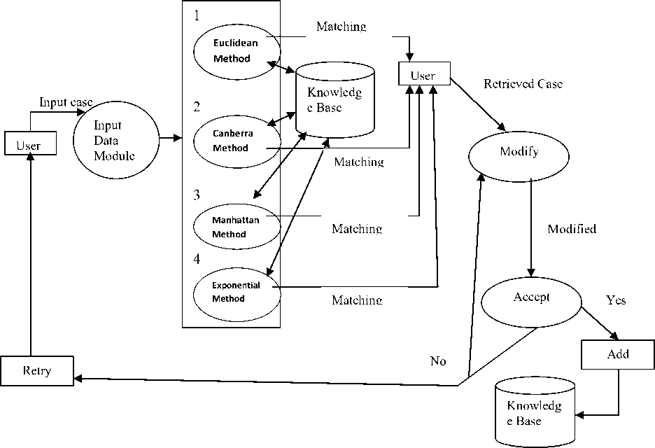
Fig 2: Software quality prediction system with four distance functions

VIII. Estimation criteria

The fundamental requirement of evaluating and validating the methodology for the accuracy of estimations, we have used error prediction method i.e. Mean Magnitude of Relative Error (MMRE) to measure how accurate the estimations are. Relative error is the absolute error in the observations divided by its actual parameter. Improvements in accuracy of predictions and increasing the reliability of the knowledge base were a priority. The research paper present the results obtained when applying the case-based reasoning model to the data set. The accuracy of estimates is evaluated by using the magnitude of relative error (MRE) defined as:

MRE= │Actual_Parameter– Targeted_Parameter│ Actual Parameter

IX. Research category

Case-based reasoning (CBR) is most popular machine learning technique. A CBR system is an expert system that aims at finding solutions to a new problem based on previous experience. Therefore we can classify this research work as an “expert system” because system consists of a knowledge base and a software module called the inference engine to perform inferences from the knowledge base. These inferences are communicated to the user. Figure.3 shows the components of an expert system [18].

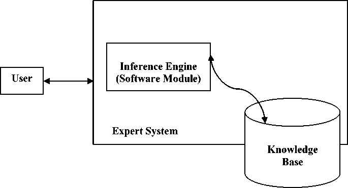
Fig 3: Components of an Expert System

X. Experimental analysis and results

The main objective of this prediction system is to help development of good quality software. The purpose of the paper is also to explore how case-based reasoning technique can support decision-making and help control dissimilarity in software fault activities, thus ultimately enhancing software quality. Estimating reliability of upcoming software versions based on fault history the fault estimation to enhance test stage effectiveness; task of resources to fix faults, and distinguishing faulty software modules from non-faulty ones. We have developed a case-based reasoning model and have validated it upon student data (see figure 2). 150 data set has been used in this research, where 80% data have used for model development and 20% data has been used for validation of the model (not used for building of models). Five consecutive experiments were performed and result with respect to development time (MRE w.r.t. Dev_Time) has been predicted because development time or time constraint affects the quality level (acceptable limit less than or equal to 10%). Second, the mean error of each record set is calculated for each attributes of nearest data in the knowledge base (acceptable limit less than or equal to 10%). It was observed that predictions are 71.198% and 92.664% of the cases within 10% error using Euclidean and Exponential method and predictions are 67.998% and 87.328% of the cases within 10% error using the Manhattan method, while predictions are 43.864% and 57.332% of the cases within 10% error using Canberra method (See table 7). The results are coming quite good when Euclidean and Exponential method has been used. Therefore we can conclude that Euclidean and Exponential both are good for error calculation in comparison to Manhattan and Canberra while applying CBR technique. In this research we have shown the strong motivation behind the use of CBR as a tool for solving the problem which has been given as a snapshot in this paper. Snapshot results can be seen in the table 2 of first row which is bold given in the appendix as an example. It seems that the model is application-based and it is very easy to extend this model to a theoretical case-based reasoning. As we know that CBR can not develop robustly without theoretical support.

Table 2: The Mean and Std. Deviation of Error with respect to Dev_time using four similarity functions (Experiment no 1).

Output	Name of Similarity Functions	Mean	Std. Deviation
Error w.r.t.	Euclidean	8.6667	15.97484
Dev_Time	Manhattan	11.3000	15.32217
	Canberra	19.9667	21.34040
	Exponent	8.6667	15.97484
Distance (Error)	Euclidean	4.5487	3.96596
	Manhattan	5.4452	4.94870
	Canberra	9.2740	7.08273
	Exponent	4.5487	3.96596

Table 3: The Mean and Std. Deviation of Error with respect to Dev_time using four similarity functions (Experiment no 2).

Output	Name of Similarity Functions	Mean	Std. Deviation
Error w.r.t . Dev_Time	Euclidean	8.1000	11.90291
	Manhattan	9.0333	13.31446
	Canberra	24.3333	23.88093
	Exponent	8.1000	11.90291
Distance (Error)	Euclidean	3.1643	2.49421
	Manhattan	5.1690	3.94575
	Canberra	9.0093	6.98985
	Exponent	3.1643	2.49421

Table 4: The Mean and Std. Deviation of Error with respect to Dev_time using four similarity functions (Experiment no 3).

Output	Name of Similarity Functions	Mean	Std. Deviation
Error w.r.t . Dev_Time	Euclidean	8.7667	12.77282
	Manhattan	9.7333	15.70402
	Canberra	18.5000	21.76006
	Exponent	8.7667	12.54697
Distance (Error)	Euclidean	4.2693	4.44246
	Manhattan	5.3343	5.11041
	Canberra	7.3387	6.52675
	Exponent	4.2693	4.44246

Table 5: The Mean and Std. Deviation of Error with respect to Dev_time using four similarity functions (Experiment no 4).

Output	Name of Similarity Functions	Mean	Std. Deviation
Error w.r.t . Dev_Time	Euclidean	7.3667	11.27855
	Manhattan	6.7667	10.88714
	Canberra	24.4333	25.56086
	Exponent	7.3667	11.27855
Distance (Error)	Euclidean	4.0380	5.33121
	Manhattan	4.6987	4.22531
	Canberra	9.6307	8.15100
	Exponent	4.0380	5.33121

Table 6: The Mean and Std. Deviation of Error with respect to Dev_time using four similarity functions (Experiment no 5).

Output	Name of Similarity Functions	Mean	Std. Deviation
Error w.r.t . Dev_Time	Euclidean	7.7333	15.17924
	Manhattan	8.1667	15.34226
	Canberra	19.9667	21.34040
	Exponent	7.7333	15.17924
Distance (Error)	Euclidean	4.6903	3.95750
	Manhattan	5.2573	4.22976
	Canberra	10.0407	7.28614
	Exponent	4.6903	3.95750

Table 7: “The Average (%) of 150 data set in five consecutive experiment results using four similarity functions using CBR technique.”

Experi ment from 1 to 5

Euclidean Method

Manhattan Method

Canberra Method

Exponential Method

MRE w.r.t Dev_Time within (10% )

Acceptable%E rror (Acceptable Limit 10%)

MRE w.r.t Dev_Ti me within(1 0%)

%Error (Acceptable Limit 10%)

MRE w.r.t Dev_Tim e within(10 %)

%Error (Acceptable Limit 10%)

MRE w.r.t Dev_Tim e within(10 %)

%Error

(Acceptable Limit 10%)

1-5

71.198%

92.664%

67.998%

87.328%

43.864%

57.332%

71.198%

92.664 %

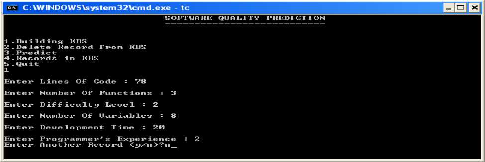
Snapshot 1: Building the knowledge base

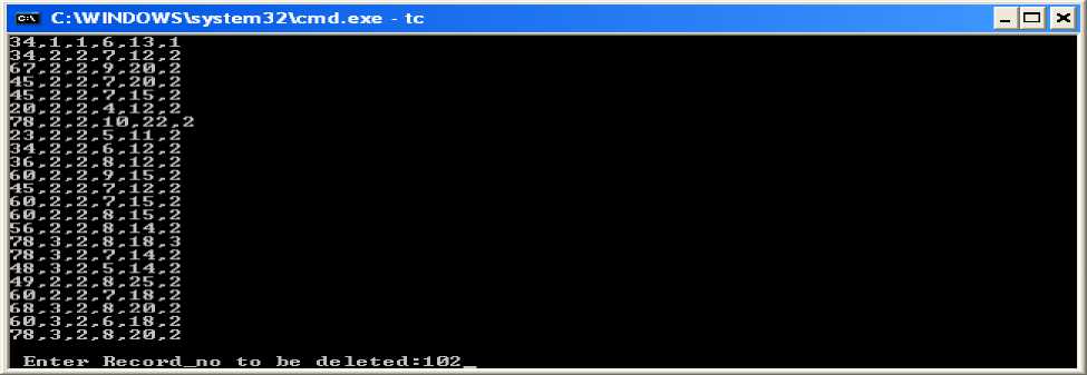
Snapshot 2: Deletion of duplicate record set from KBS for reducing the maintenance cost.

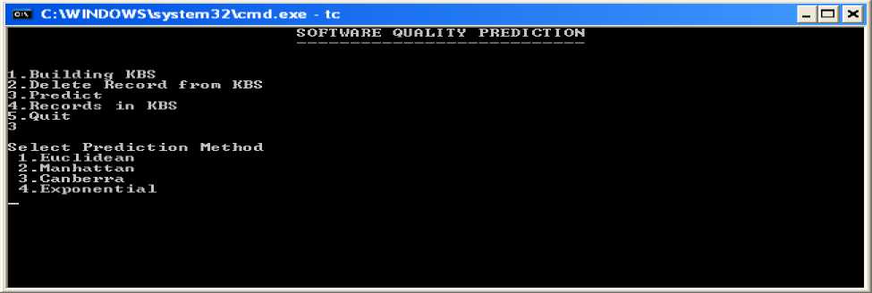
Snapshot 3: Selection of similarity Function for error prediction

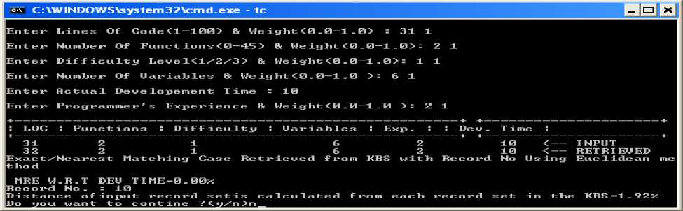
Explanation: Snapshot 4. Accuracy using Euclidean Method (Exact/Nearest mathing case retrieved from the knowledge base along with a record no as well as MRE w.r.t Dev_Time value=0%. In this research magnitude of relative error is calculated with the help of dependent variable I, e development time. It can be seen in the form of output where the input parameter given by the user during run time and getting the result from the knowledge base as a retrieved case in which dependent variable is development time is same. In this case rest of the parameters have been matched except LOC which is retrieved from the knowledge base. We also display the distance of the input record set is calculated for each attributes of nearest data in the knowledge base (KBS) in the form of error (See Table 2 of row one which is bold given in appendix)

Explanation: Snapshot 5. Accuracy using Manhattan Method (Exact/Nearest mathing case retrieved from knowledge base along with record no as well as MRE w.r.t Dev_Time value=0%. In this research magnitude of relative error is calculated with the help of dependent variable I, e development time. It can be seen in the form of output where the input parameter given by the user during runs time and getting the result from the knowledge base as a retrieved case in which dependent variable is development time is same. In this case rest of the parameters have been matched except LOC which is retrieved from the knowledge base. We also display the distance of the input record set is calculated for each attributes of nearest data in the knowledge base (KBS) in the form of error (See Table 2 of row one which is bold given in appendix)

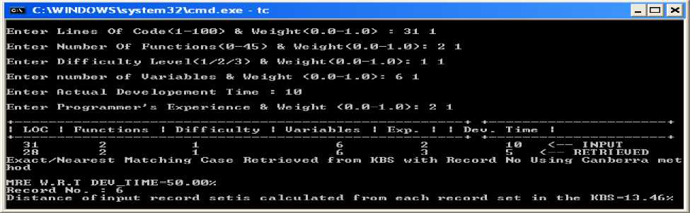
Explanation: Snapshot 6: Accuracy using Canberra Method (Exact/Nearest mathing case retrieved from the knowledge base along with record no as well as MRE w.r.t dev_Time value=50%. In this research magnitude of relative error is calculated with the help of dependent variable I, e development time. It can be seen in the form of output where the input parameter given by the user during run time and getting the result from the knowledge base as a retrieved case in which dependent variable is development time is not same as stored in the knowledge base as well as rest of the parameters are not exact matched, it is a nearest matching case which has been retrieved from the knowledge base. We also display distance of input record set is calculated for each attributes of nearest data in the knowledge base (KBS) in the form of error (See Table 2 of row one which is bold given in appendix).

Explanation: Snapshot 7. Accuracy using Exponential Method (Exact/Nearest mathing case retrieved from knowledge base along with record no as well as MRE w.r.t Dev_Time value=0%. In this research magnitude of relative error is calculated by the help of dependent variable i,e development time. It can be seen in the form of output where the input parameter given by the user during run time and getting the result from the knowledge base as a retrieved case in which dependent variable is development time is same. In this case rest of the parameters have been matched except LOC which is retrieved from the knowledge base. We also display distance of input record set is calculated for each attributes of nearest data in the knowledge base (KBS) in the form of error (See Table 2 of row one which is bold given in appendix).

XI. Advantages of this research

The software is compiled using Turbo C++ 3.0 and hence it is very compact and standalone, It can be readily deployed on any low configuration system and it would not impact its performance, as it does not rely on external runtimes and DLL’s like the .NET programs rely on. The software is a console based application and thus does not use the GUI functions of the operating System, which makes it very fast in execution.

The biggest advantages of this research has given below:

a) A Knowledge base (KBS) is created and maintained to store the cases as a different attributes of the software against which the matching process has to be performed.
b) The objective is to predict the quality of the software project accurately and use the results in future predictions.
c) The matching has done using various similarity measures like Euclidean, Manhattan, Canberra, Exponential.
d) The prediction is based upon Case-Based Reasoning (CBR) technique. Because CBR takes minimum time in comparison to other AI approach like Neural Network (NN) and Genetic Algorithm (GA). But for accuracy the data requirement for CBR, NN, GA are high [23].
e) New features and functionalities can be added easily to the existing system to satisfy the future requirements for example easy to extend.
f) The advantages of this research work are a result-oriented because CBR systems use nearest neighbor algorithm for retrieval of cases from the Knowledge base.
g) Improving the quality of the software through early prediction of error patterns.
h) Removing the duplicate record set from the KBS for reducing the maintenance cost.
i) This technique can be successfully applied to fault diagnosis for customer service support.
j) CBR systems can use existing solution and adapt it to the current situation.
k) To add new record set to CBR system, a user only needs to add new cases to the system.

XII. Conclusions

The main contribution of this paper is a use of case-based reasoning as an expert system for predicting the software fault in a software module. After developing the case-based reasoning model (see figure 2) we validated it with part of the data set. In this research work four distance functions the Euclidean, Canberra, Exponential and Manhattan method were taken into consideration in terms of percentage of errors generated during execution of programs. For their efficacy in determining errors, the low error programs detected by these methods may help to design error free programs. If the error estimation is less than 10% then the input record set is auto saved to the knowledge base. Once the result is predicted it is added to the database to enhance the accuracy of future predictions. Only those results are added that give an error of 10% or less. But if the error estimation is more than 10% then the input record set must be revised then save to the knowledge base for future solutions. These data can be safely classified as high quality data. In the current analysis, the accuracy performed by all four distance functions which is given in the tabular form (See appendix) while using CBR technique. Also it can be seen in the form of a snapshot (See snapshot 4 through snapshot 7). And a result is derived where acceptable range is within 10%. Snapshot 4, 5, 6 and 7 shows the accuracy comparisons of different distance functions. The average (%) of the 150 data set in five consecutive experiment results using four similarity functions using CBR technique shown in table 7. We have also calculated the mean and standard deviation of each experiment results using these similarity functions (see table 2 through 6).

XIII. Future scope

Through empirical investigations and literature reviews conducted as part of this research work, we anticipate a promising future where there are further research opportunities for evaluating the application of case-based reasoning in software quality prediction and software testing. The long term goal of the research is as follows:

1. Use of neural network and/or fuzzy logic model for software quality prediction.
2. Addition of new parameters: Additional fields can be added to the record set so as to incorporate the dependency of the prediction if any, on these parameters. Till now, only those parameters were considered that had more dependency.
3. Addition of new similarity measures: Apart from Euclidean, Canberra, Exponential and Manhattan methods other similarity measures can be used to find similar cases. For example Chebychev method. Choice in the use of similarity measure adds flexibility to the system and allows to compare among the methods.

APPENDIX A

Table 1: Comparative Analysis of Error Prediction with four distance functions using CBR technique (Experiment One).

Id	Euclidean Method		Manhattan Method		Canberra Method		Exponential Method
Id	MRE w.r.t Dev_Time within (10% )	%Error (Acceptable Limit 10%)	MRE w.r.t Dev_Ti me within(1 0%)	%Error (Acceptable Limit 10%)	MRE w.r.t Dev_ Time within (10%)	%Error (Acceptable Limit 10%)	MRE w.r.t Dev_Ti me within(1 0%)	%Error (Acceptable Limit 10%)
1	25	5.68	25	5.68	25	5.68	25	5.68
2	0.0	5.71	0.0	11.43	50	14.29	0.0	5.71
3	0.0	8.93	0.0	8.93	33	16.07	0.0	8.93
4	20	6.0	0.0	0.0	0.0	0.0	20	6.0
5	0.0	1.89	0.0	1.89	0.0	1.89	0.0	1.89
6	0.0	2.86	0.0	2.86	0.0	5.71	0.0	2.86
7	0.0	5.45	0.0	5.45	33	5.45	0.0	5.45
8	7	0.0	23	2.38	23	7.14	7	0.0
9	20	2.13	20	2.13	20	2.13	20	2.13
10	25	7.14	25	7.14	0.0	0.0	25	7.14
11	0.0	2.63	0.0	5.41	50	18.92	0.0	2.63
12	0.0	0.0	0.0	0.0	13	12.50	0.0	0.0
13	0.0	2.13	0.0	2.13	0.0	10.64	0.0	2.13
14	75	3.57	0.0	17.86	0.0	17.86	75	3.57
15	33	4.17	33	4.17	33	4.17	33	4.17
16	0.0	3.45	30	5.17	60	20.69	0.0	3.45
17	0.0	3.33	25	8.33	50	13.33	0.0	3.33
18	0.0	6.67	0.0	3.33	50	13.33	0.0	6.67
19	16	7.46	16	10.45	16	10.45	16	7.46
20	0.0	1.49	23	7.46	23	7.46	0.0	1.49
21	0.0	4.44	0.0	4.44	0.0	4.44	0.0	4.44
22	0.0	20.0	50	0.0	0.0	0.0	0.0	20.0
23	0.0	5.08	0.0	5.08	0.0	11.86	0.0	5.08
24	11	11.76	44	21.32	44	21.32	11	11.76
25	8	3.45	25	5.17	16	10.34	8	3.45
26	0.0	2.67	0.0	1.33	0.0	1.33	0.0	2.67
27	20	2.94	0.0	2.94	0.0	11.76	20	2.94
28	0.0	0.97	0.0	0.97	0.0	0.0	0.0	0.97
29	0.0	4.46	0.0	4.46	0.0	4.46	0.0	4.46
30	0.0	0.0	0.0	0.0	60	25	0.0	0.0

70% 96.66% 60% 86.66% 43% 50% 70% 96.66%

Table 2: Comparative Analysis of Error Prediction with four distance functions using CBR technique (Experiment Two)

Id	Euclidean Method		Manhattan Method		Canberra Method		Exponential Method
Id	MRE w.r.t Dev_Tim e within (10% )	%Error (Acceptable Limit 10%)	MRE w.r.t Dev_Ti me within(1 0%)	%Error (Acceptable Limit 10%)	MRE w.r.t Dev_ Time within (10%)	%Error (Acceptable Limit 10%)	MRE w.r.t Dev_Ti me within(1 0%)	%Error (Acceptable Limit 10%)
1	0.0	1.92	0.0	1.92	50	13.46	0.0	1.92
2	40.0	3.70	50	12.35	40.0	3.70	40.0	3.70
3	6.0	1.20	0.0	6.02	6.0	1.20	6.0	1.20
4	0.0	10.0	0.0	10.0	0.0	10.0	0.0	10.0
5	0.0	0.0	0.0	4.69	0.0	4.69	0.0	0.0
6	7.0	5.0	15.0	1.67	23.0	11.67	7.0	5.0
7	0.0	2.78	16	1.39	16	13.89	0.0	2.78
8	25	2.17	25	2.17	25	2.17	25	2.17
9	0.0	5.41	0.0	5.41	0.0	5.41	0.0	5.41
10	0.0	3.17	0.0	3.17	33.0	4.76	0.0	3.17
11	25	6.38	25	6.38	25	0.0	25	6.38
12	0.0	6.90	0.0	6.90	0.0	6.90	0.0	6.90
13	28	2.86	0.0	14.29	28	22.86	28	2.86
14	25	2.38	37.0	11.90	37.0	11.90	25	2.38
15	15	1.64	15	0.0	53.0	21.31	15	1.64
16	0.0	6.25	0.0	6.25	60	12.50	0.0	6.25
17	0.0	5.17	0.0	5.17	0.0	3.45	0.0	5.17
18	0.0	0.0	0.0	10.26	0.0	10.26	0.0	0.0
19	0.0	0.0	0.0	0.0	33	11.76	0.0	0.0
20	8.0	0.0	8.0	0.0	66	16.42	8.0	0.0
21	15	3.03	15	3.03	69	15.15	15	3.03
22	9.0	2.94	9.0	2.94	63	17.65	9.0	2.94
23	7.0	0.0	7.0	0.0	7.0	0.0	7.0	0.0
24	0.0	4.67	0.0	4.67	20.0	1.87	0.0	4.67
25	0.0	5.36	0.0	5.36	0.0	5.36	0.0	5.36
26	33.0	5.32	33.0	5.32	0.0	4.26	33.0	5.32
27	0.0	0.98	0.0	2.94	0.0	2.94	0.0	0.98
28	0.0	3.45	16	8.62	16	8.62	0.0	3.45
29	0.0	2.25	0.0	2.25	0.0	1.12	0.0	2.25
30	0.0	0.0	0.0	10.0	60	25	0.0	0.0

76% 100% 70% 86.66% 46.66% 60% 76% 100%

Table 3: Comparative Analysis of Error Prediction with four distance functions using CBR technique (Experiment Three)

Id	Euclidean Method		Manhattan Method		Canberra Method		Exponential Method
Id	MRE w.r.t Dev_Time within (10%)	%Error (Acceptable Limit 10%)	MRE w.r.t Dev_Ti me within (10%)	%Error (Acceptable Limit 10%)	MRE w.r.t Dev_ Time within (10%)	%Error (Acceptable Limit 10%)	MRE w.r.t Dev_Ti me within (10%)	%Error (Acceptable Limit 10%)
1	25	5.68	25	5.68	25	5.68	25	5.68
2	0	3.33	0	3.33	0	3.33	0	3.33
3	20	6.67	0	11.11	20	6.67	20	6.67
4	0	0	0	0	0	0	0	0
5	0	1.64	0	4.92	0	1.64	0	1.64
6	0	0	0	0	0	0	0	0
7	0	11.11	0	11.11	0	11.11	0	11.11
8	25	0	0	5.41	0	13.51	25	0
9	0	5.17	0	5.17	73	20.69	0	5.17
10	0	0	0	0	0	0	0	0
11	25	20	25	20	25	8	25	20
12	33	5	66	17.50	33	5	33	5
13	42	12.50	42	12.50	42	5	42	12.50
14	0	0	0	0	0	0	0	0
15	25	9.09	0	9.09	50	18.18	25	9.09
16	0	3.23	0	3.23	13	9.68	0	3.23
17	0	4.88	0	9.76	0	4.88	0	4.88
18	0	2.78	0	2.78	0	2.78	0	2.78
19	0	2.60	0	3.90	0	3.90	0	2.60
20	0	4.29	0	4.29	0	2.86	0	4.29
21	11	0	11	0	16	10.45	11	0
22	7	1.79	7	1.79	64	16.07	7	1.79
23	8	5.26	8	5.26	16	8.77	8	5.26
24	25	1.92	25	1.92	50	23.08	25	1.92
25	0	1.37	0	1.37	0	1.37	0	1.37
26	0	4.84	25	1.61	41	12.90	0	4.84
27	0	3.41	0	5.68	0	1.14	0	3.41
28	22	3.57	22	3.57	22	5.36	22	3.57
29	20	7.95	20	7.95	40	15.91	20	7.95
30	0	0	16	1.10	16	2.20	0	0

63.33% 90% 66.66% 86.66% 46.66% 70% 63.33% 90%

Table 4: Comparative Analysis of Error Prediction with four distance functions using CBR technique (Experiment Four)

Id	Euclidean Method		Manhattan Method		Canberra Method		Exponential Method
Id	MRE w.r.t Dev_Time within (10%)	%Error (Acceptable Limit 10%)	MRE w.r.t Dev_Time within (10%)	%Error (Acceptable Limit 10%)	MRE w.r.t Dev_Time within (10%)	%Error (Acceptable Limit 10%)	MRE w.r.t Dev_Time within (10%)	%Error (Acceptable Limit 10%)
1	0	2.13	0	2.13	0	2.13	0	2.13
2	0	11.11	0	6.67	60	13.33	0	11.11
3	0	0	0	4.69	0	4.69	0	0
4	0	1.96	0	9.80	73	23..53	0	1.96
5	0	5.13	0	10.26	0	10.26	0	5.13
6	0	0	0	4.69	0	4.69	0	0
7	0	3.23	0	3.23	0	3.23	0	3.23
8	0	0	0	7.69	0	0	0	0
9	20	2.63	20	0	0	27.03	20	2.63
10	25	7.41	0	8.64	25	8.64	25	7.41
11	13	2.94	0	0	73	17.65	13	2.94
12	0	2.38	0	2.38	0	2.38	0	2.38
13	0	28	0	20	20	0	0	28
14	0	3.51	0	1.75	33	8.77	0	3.51
15	40	2.94	40	2.94	0	11.76	40	2.94
16	0	2.13	0	2.13	60	17.02	0	2.13
17	0	3.23	0	3.23	25	11.29	0	3.23
18	26	8.33	26	8.33	55	22.92	26	8.33
19	20	7.37	20	7.37	20	7.37	20	7.37
20	0	6.25	0	4.69	50	18.75	0	6.25
21	7	1.79	15	8.93	69	17.86	7	1.79
22	25	5.13	25	6.41	25	5.13	25	5.13
23	18	3.45	18	3.45	18	3.45	18	3.45
24	0	2.86	0	2.86	8	2.86	0	2.86
25	20	5.88	0	2.94	0	11.76	20	5.88
26	7	1.35	7	1.35	7	1.35	7	1.35
27	0	0	16	1.10	16	3.30	0	0
28	0	0	16	3.30	16	3.30	0	0
29	0	0	0	0	20	0	0	0
30	0	0	0	0	60	25	0	0

70% 93.33% 70% 93.33% 40% 56.66% 70% 93.33%

Table 5: Comparative Analysis of Error Prediction with four distance functions using CBR technique (Experiment Five)

Id	Euclidean Method		Manhattan Method		Canberra Method		Exponential Method
Id	MRE w.r.t Dev_time within (10%)	%Error (Acceptable Limit 10%)	MRE w.r.t Dev_Ti me within (10%)	%Error (Acceptable Limit 10%)	MRE w.r.t Dev_ Time within (10%)	%Error (Acceptable Limit 10%)	MRE w.r.t Dev_Ti me within (10%)	%Error (Acceptable Limit 10%)
1	0	1.35	0	4.05	25	5.68	0	1.35
2	0	4.88	0	4.88	50	14.29	0	4.88
3	0	1.69	0	1.67	33	16.07	0	1.69
4	16	9.62	25	7.69	0.0	0.0	16	9.62
5	0	0	0	0	0.0	1.89	0	0
6	0	0	0	7.69	0.0	5.71	0	0
7	66	11.11	66	11.11	33	5.45	66	11.11
8	25	0	0	16.67	23	7.14	25	0
9	42	11.11	42	11.11	20	2.13	42	11.11
10	0	2.67	0	2.67	0.0	0.0	0	2.67
11	0	12.50	0	12.50	50	18.92	0	12.50
12	16	10.34	16	8.62	13	12.50	16	10.34
13	0	2	0	2	0.0	10.64	0	2
14	0	9.30	0	9.30	0.0	17.86	0	9.30
15	7	1.49	7	1.49	33	4.17	7	1.49
16	0	6.25	0	6.25	60	20.69	0	6.25
17	0	2.17	0	2.17	50	13.33	0	2.17
18	7	3.70	0	1.85	50	13.33	7	3.70
19	0	6.32	0	1.05	16	10.45	0	6.32
20	0	4.11	20	1.37	23	7.46	0	4.11
21	0	3.30	0	3.30	0.0	4.44	0	3.30
22	0	11.81	0	11.81	0.0	0.0	0	11.81
23	16	7.14	16	7.14	0.0	11.86	16	7.14
24	9	4.26	9	4.44	44	21.32	9	4.26
25	0	2.22	0	2.22	16	10.34	0	2.22
26	0	1.96	0	1.96	0.0	1.33	0	1.96
27	28	5.66	28	5.66	0.0	11.76	28	5.66
28	0	2.78	0	2.78	0.0	0.0	0	2.78
29	0	0.97	0	0.97	0.0	4.46	0	0.97
30	0	0	16	3.30	60	25	0	0

76.66% 83.33% 73.33% 83.33% 43% 50% 76.66% 83.33%

APPENDIX B

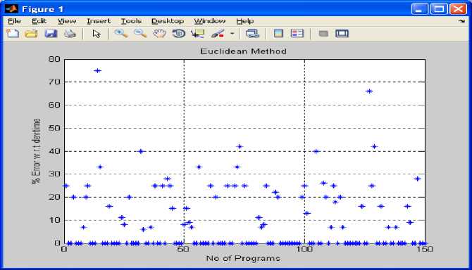
Fig 1: shows number of programs versus % error predicted with respect to development time using Euclidean method on the basis of experiment 1 to experiment 5

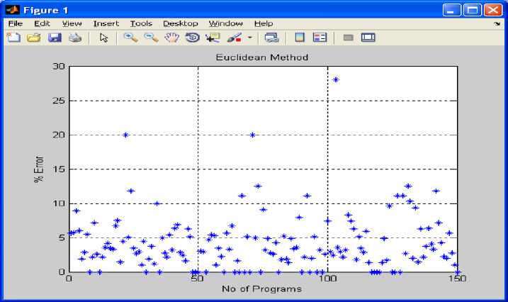
Fig 2: shows number of programs versus % error using Euclidean method on the basis of table 1 to table 5.

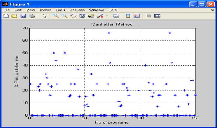
Fig 3: shows number of programs versus % error predicted with respect to development time using Manhattan method on the basis of table 1 to table 5.

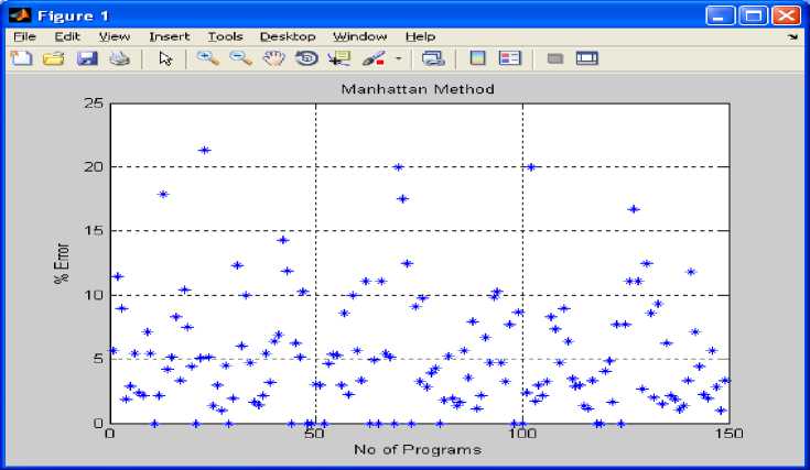
Fig 4: shows number of programs versus % error using Manhattan method on the basis of table 1 to table 5.

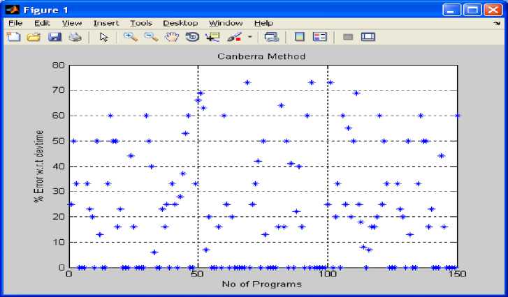
Fig 5: shows number of programs versus % error predicted with respect to development time using Canberra method on the basis of table 1 to table 5.

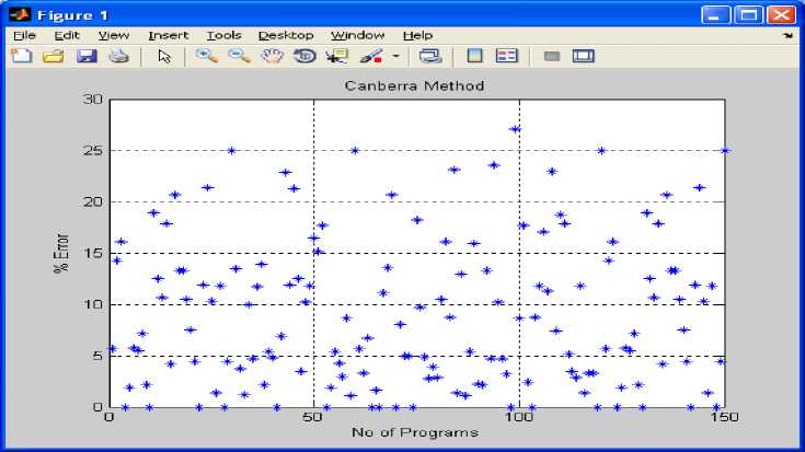
Fig 6: shows number of programs versus % error with respect to development time using Manhattan method on the basis of table 1 to table 5.

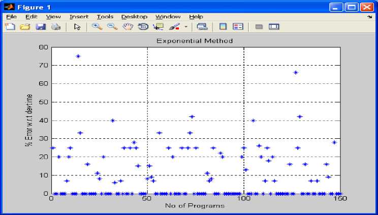
Fig 7: shows number of programs versus % error predicted with respect to development time using Exponential method on the basis of table 1 to table 5.

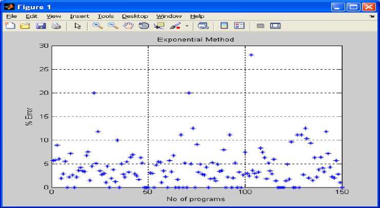
Fig 8: shows number of programs versus % error using Exponential method on the basis of table 1 to table 5.

Список литературы Machine Learning and Software Quality Prediction: As an Expert System

G. Kadoda, M Cartwright, L Chen, and M. Shepperd. (2000), “Experiences Using Case- Based Reasoning to Predict Software Project Effort”, In Proceeding of EASE, p. 23-28, Keele, UK.
I. Myrtveit and E. Stensrud. (1999), “A Controlled Experiment to Assess the Benefits of Estimating with Analogy and Regression Models”, IEEE transactions on software Engineering, Vol 25, no. 4, pp. 510-525.
K. Ganeasn, T.M. Khoshgoftaar, and E. Allen. (2000), “Case-based Software Quality Prediction”, International journal of Software Engineering and Knowledge Engineering, 10 (2), pp. 139-152.
Bob Hughes & Mike Cotterell “software Project Management”, Tata McGraw-Hill.
Shi Zhong,Taghi M.Khoshgoftaar and Naeem Selvia “Unsupervised Learning for Expert-Based Software Quality Estimation”.Proceeding of the Eighth IEEE International Symposium on High Assurance Systems Engineering (HASE’04).
Ekbal Rashid, Srikanta Patnaik, Vandana Bhattacherjee “A Survey in the Area of Machine Learning and Its Application for Software Quality Prediction” has been published in ACM SigSoft ISSN 0163-5948, volume 37, number 5, September 2012, http://doi.acm.org/10.1145/2347696.2347709 New York, NY, USA.
M. J. Khan, S. Shamail, M. M Awais, and T. Hussain, “Comparative study of various artificial intelligence techniques to predict software quality” in proceedings of the 10th IEEE multitopic conference, 2006, INMIC 06, PP 173-177, Dec 2006.
S. Becker, L. Grunske, R. Mirandola, and S. Overhage, “ Performance prediction of component-based systems a survey from an engineering perspective”, In architechture systems with Trust-worthy components, Vol 3938 of LNCS, Springer, 2006.
Ekbal Rashid, Srikanta Patnaik, Vandana Bhattacherjee “Enhancing the accuracy of case-based estimation model through Early Prediction of Error Patterns” proceedings published by the IEEE Computer Society 10662 Los Vaqueros Circle Los Alamitos, CA, in International Symposium on Computational and Business Intelligence (ISCBI 2013), New Delhi, 24~26 Aug 2013 ISBN 978-07695-5066-4/13 IEEE, DOI 10.1109/ISCBI.2013.
Aamodt, A. and E. Plaza, Case-based reasoning: foundational issues, methodical variations and system approaches. AI Communications 7(1), 1994.
M. M.T. Thwin and T.S. Quah, “Application of neural network for predicting software development faults using object-oriented design metrics” in proceeding of the 9th International Conference on neural information processing, ICONIP 02 Vol. 5, 2002.
D. Grosser, H. A. Sahraoui, and P. Valtchev, “Analogy-based software quality prediction”, in 7th Workshop on Quantitative Approaches in Object-Oriented Software Engineering, QAOOSE 03, June 2003.
T.W. Lioa, and Z. Zhang, “Similarity measures for retrieval in Case-Based Reasoning Systems” Applied Artificial Intelligence, Vol. 12, 1998, 267-288.
Venkata U.B.Challagulla et al ”A Unified Framework for Defect data analysis using the MBR technique”. Proceeding of the 18th IEEE International Conference on Tools with Artificial Intelligence (ICTAI’06).
Lance, G. N.; Williams, W. T. (1966). "Computer programs for hierarchical polythetic classification ("similarity analysis")."Computer Journal 9 (1): 60–64. doi:10.1093/comjnl/9.1.60.
Lance, G. N.; Williams, W. T. (1967). "Mixed-data classificatory programs I.) Agglomerative Systems". Australian Computer Journal: 15–20.
Stephen H. Kan Metrics and Models in Software Quality Engineering, second edition by Pearson.
Donald A. Waterman A guide to Expert Systems, First Impression, 2008, Pearson.
Du Zhang, Jeffrey J. P. Tsai “Advances in Machine Learning Applications in Software Engineering” Idea Group Publishing.
L. C. Briand, W. L.Melo and J. Wust. “Assessing the applicability of fault-proneness models across object-oriented software projects” IEEE Transactionson Software Engineering, 28(7): 706-720, July 2002.
T. M. Khoshgoftaar and N. Seliya. Analogy-based practical classification rules for software quality estimation Empirical Software Engineering Journal, 8(4):325-350, December 2003.
Begum, S. Ahmed, M.U.; Funk, P.; Ning Xiong; “Folke, M.Sch. of Innovation, Design & Eng., Malardalen Univ., Vasteras, Sweden, Published in Systems, Man, and Cybernetics, Part C: Applications and Reviews, IEEE Transactions on (Volume:41, Issue: 4), July 2011, ISSN :1094-6977, 10.1109/TSMCC.2010.2071862.
“A Survey of measurement-based software quality prediction techniques” Technical Report, Lums, Dec 2007.

Еще

Статья научная

Machine Learning and Software Quality Prediction: As an Expert System

Текст научной статьи Machine Learning and Software Quality Prediction: As an Expert System

II. Background and related work

III. Learning/prediction system

IV. Software quality

V. Selection of distance functions

VI. Methodology

VIII. Estimation criteria

IX. Research category

X. Experimental analysis and results

XI. Advantages of this research

XII. Conclusions

XIII. Future scope

Список литературы Machine Learning and Software Quality Prediction: As an Expert System