Machine learning applied to cervical cancer data

Cervical Cancer is cancer arising from the cervix. It arises due to the abnormal growth of cells and spreads to other parts of the body. It is fatal most of the time. HPV causes most of the cases (90 %). The data is cleaned, and outliers were taken care. Smoking is also considered as one of the main causes for cervical cancer. Longterm use of Oral contraceptive pills can also cause cancer. Also having multiple pregnancies can cause cervical cancer. Usually it is very difficult to identify cancer at early stages. The early stages of cancer are completely free of symptoms. It is only during the later stages of cancer that symptoms appear. We can use machine learning techniques to predict if a person has cancer or not.

Around the globe, around a quarter of million people die owing to cervical cancer. Screening and different deterministic tests confuse the available Computed Aided Diagnosis (CAD) to treat the patient correctly for the cancer. Several factors for cancer include age, number of sexual partners, age of first sexual intercourse,

* Corresponding author.

number of pregnancies, smoking habits, hormonal, STD’s detected in the patient and any diagnosis performed for cancer and diseases like HPV (Human papillomavirus) and CIN (Cervical intraepithelial neoplasia). For cervical cancer, the screening methods include cytology, Schiller, Hinselmann and the standard biopsy test. Each test is carried out to detect the presence of cervical cancer. Different models are tried on the dataset. Fine tuning of the parameters is done. The performance of Different models are compared. And finally, the best models are recommended that can be used to predict cancer[7,6].

2.    Data Exploration

The data has 36 columns out of which 4 columns are the target columns of the four tests conducted which determine if the patient has cancer or not. The remaining 32 columns are the several factors that may lead to the cervical cancer. These factors play a significant role to identify the cancer in patient. We have made several data visualizations to check the instances of these factors.

After looking the data, we found several question mark signs (?) present in the columns. For modelling purpose, the question mark’s need to be replaced with some meaningful values. We decided to replace all the question marks with median value of the column[11,14].

For making better predictions we replaced the value 1,2,3,4 by 1 meaning that the patient has cancer and 0 meaning that the patient does not have cancer[15,8]

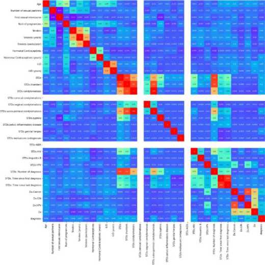
Fig.1. Correlation Plot of all the Columns.

The below heatmap, displays all the factors responsible for cervical cancer and their correlation with each other. The last column ‘diagnosis’ represents the target column. We have created this target column from the available four target columns for modelling purpose.[9,10]

3.    Methodology

In order to build the model, three different classifier techniques are used. Decision tree, K-nearest neighbor and random forest. During the initial analysis it was found that the dataset is biased hence k-fold crossvalidation is done. For k-nearest neighbor dataset is split 50-50. Feature selection is done, and the selected features are used for prediction. For decision tree and random forest, the data is split 25-75. Parameter tuning is done to get the best predictions with optimal evaluation scores.[3,5] We also used Hill climbing Algorithm for feature selection. The algorithm is a mathematical optimization that use heuristic search in the felid of Artificial Intelligence. Following are steps how the algorithm does a feature selection.

Step 1:  Make initial state as current state after evaluating the initial state

Step 2:  Run the loop till there are no features present which can be applied to current state.

• a)    Select a feature that has not been yet applied to the current state and apply it to produce a new state.

• b)    Perform these to evaluate new state

• i.    If the current state is a goal state, then stop and return success.

• ii.    If it is better than the current state, then make it current state and proceed further.

• iii.    If it is not better than the current state, then continue in the loop until a solution is found.

• 3.1.    K-Nearest Neighbor classifier

Step 3: Exit

Confusion matrix, classification error rate, Recall, F1score are used to evaluate different models. AUC curve is used to evaluate the model and is used to select the best model by parameter tuning.

For the nearest neighbor K-fold cross validation is used. Ap- propriate k value is selected based on the formula sqrt(N)/2 which gives us 10.3. The sample size of the training dataset is chosen to be 429. After running several models the value of K is chosen as 5. Euclidean distance method is used to calculate the distance between two values. The result for the k-fold cross validation technique is shown below.

[fold 0] score: 0.8023255814

[fold 1] score: 0.9302325581

[fold 2] score: 0.8720930233

[fold 3] score: 0.9186046512

[fold 4] score: 0.9186046512

[fold 5] score: 0.9418604651

[fold 6] score: 0.9418604651

[fold 7] score: 0.8604651163

[fold 8] score: 0.8823529412

[fold 9] score: 0.9529411765

Fig.2. K-fold Cross Validation

Lower value of k is biased. Higher values of k is less biased but it can show variance. Since k=5 which is neither less nor more. Or the k-nearest neighbour the dataset is split 50-50. Feature selection is done which help us to select the features that will improve the prediction. The 25 features selected for the predictions are

Table 1. Features selected for K-Nearest Neighbor Classifier

Features selected for K-Nearest Neighbour Classifier
Age	STDs (number)
Number of sexual partners	STDs:condylomatosis
First sexual intercourse	STDs:cervical condylomatosis
Num of pregnancies	STDs:vaginal condylomatosis
Smokes	STDs:vulvo-perineal condylomatosis
Smokes (years)	STDs:syphilis
Smokes (packs/year)	STDs:pelvic inflammatory disease
Hormonal Contraceptives	STDs:genital herpes
Hormonal Contraceptives (years)	STDs:molluscum contagiosum
IUD	STDs:AIDS
IUD (years)	STDs:HIV
STDs	STDs:Hepatitis B
	STDs:HPV

• 3.2.    Decision tree Classifier

• 3.3.    Random Forest Algorithm

For the decision tree classifier, the dataset is split 25%. Presort function is used for fast implication of the algorithm. To minimize the size of the tree the minimum split for sample is set at 110. Class weight is used as balanced so that it automatically adjusts the weight inversely proportional to class frequencies in the input data. Feature selection is done for decision tree classifier. The following features are selected for the prediction.

Table 2. Features selected for Decision tree Classifier

Features selected for Decision tree Classifier

STDs:AIDS	Dx:CIN
STDs:herpes STDs:cervicalcondylomatosis STDs:HPV	STDs:vaginalcondylomatosis Dx Dx:HPV
STDs: Time since first diagnosis Smokes	STDs:AIDS STDs:vulvo-perineal condylomatosis
First sexual intercourse	STDs:syphilis
IUD (years)	STDs:syphilis STDs:contagiosum

The random forest algorithm uses the training data set and generates multiple level decision tree. For the decision tree the data is split 25-75 for training and testing data. The depth of the tree is limited to 10 to make the tree less complex. After running the algorithm several times, the maximum sample split is decided to be 75. As per the inverse of frequency of input data class weight is again used as ‘balanced’ for automatic adjustment. For the random forest after we do the feature selection only 11 features are selected for prediction.

Table 2. Random Forest Algorithm

Features selected for Random Forest

STDs:HPV	Smokes
STDs:molluscum contagiosum STDs: Time since first diagnosis IUD	First sexual intercourse IUD (years) Dx:CIN
Dx	STDs:vaginal condylomatosis Dx:HPV

4.    Evaluation 4.1.    Confusion Matrix

It is a performance measurement for machine learning classification problem where output can be two or more classes. It is a table with 4 different combinations of predicted and actual values.

Actual Values

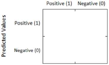
TP	FP
FN	TN

Fig.3. Confusion Matrix.

• a)    K-nearest neighbor classifier:

  
  
  

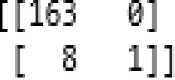
Fig.4. Confusion Matrix of K-nearest Neighbor Classifier.

According to the above confusion matrix, [1]

• •    True positive count is 163.

• •    False negative count is 0.

• •    False positive count is 8.

• •    True negative count is 1.

• b)    Decision tree classifier:

[[181 24] [ 8   2]]

Fig.5. Confusion Matrix of Decision tree Classifier.

According to the above confusion matrix, [1]

• •    True positive count is 183.

• •    False negative count is 24.

• •    False positive count is 8.

• •    True negative count is 2.

• c)    Random Forest Algorithm:

[[187 18J [ 8   2]]

Fig.6. Confusion Matrix Random Forest Algorithm.

According to the above confusion matrix, [1]

• •    True positive count is 187.

• •    False negative count is 18.

• •    False positive count is 8.

• •    True negative count is 2.

• 4.2.    Accuracy

• 4.3.    Classification Error Rate

Accuracy is one of the metric used for evaluating classification models. Informally, accuracy is the fraction of predictions our model got right. Formally, accuracy has the following definition:

Accuracy =(TP + TN)/ Total                                                               (1)

K-nearest neighbour: Accuracy of this algorithm is 95.3%.

Decision Tree Classifier: Accuracy of this algorithm is 85.11%.

Random-Forest: Accuracy of this algorithm is 87.90%

Classification error rate is one of the metric used for evaluating classification models. Informally, error rate is defined as predictions our model got it wrong.

CER = 1-accuracy                                                                          (2)

K-nearest neighbour: The classification error rate is found out to be 4.7%.

Decision Tree Classifier: The classification error rate is found out to be 14.89%.

Random-Forest: The classification error rate is found out to be 12.1%

• 4.4.    Precision, Recall and F1 Score

Out of all the classes, how much we predicted correctly. It should be high as possible. it is difficult to compare two models with low precision and high recall or vice versa. So to make them comparable, we use F-Score. F-score helps to measure Recall and Precision at the same time. It uses Harmonic Mean in place of Arithmetic Mean by punishing the extreme values more[1,2]

Precision = TP/TP+FP

Recall = TP/TP+FN

F1 Score = 2*(Recall * Precision) / (Recall + Precision)

• a)    K-nearest Neighbor:

  	precision	recall	fl-score	support
  0	0.95	1.00	0.98	163
  1	1.00	0.11	0.20	9
  avg / total	0.96	0.95	0.94	172

Fig.7. Precision Recall and F1 Score of K-nearest Neighbor Classifier.

• b)    Decision tree Classifier:

  	precision	recall	fl-score	support
  0	0.96	0.88	0.92	205
  1	0.08	0.20	0.11	10
  avg / total	0.92	0.85	0.88	215

Fig.8. Precision Recall and F1 Score of Decision tree Classifier.

• c)    Random Forest Algorithm:

• 4.5.    AUC/ROC

precision	recall fl-score support
0       0.96 1       0.10	0.91      0.94       205 0.20      0.13        10
avg / total       0.92	0.88      0.90       215

Fig.9. Precision Recall and F1 Score of Random Forest.

Area Under Curve(AUC) is one of the most widely used metrics for evaluation. It is used for binary classification problem[3,5]. AUC of a classifier is equal to the probability that the classifier will rank a randomly chosen positive example higher than a randomly chosen negative example.

• a)    K-nearest neighbor:

  

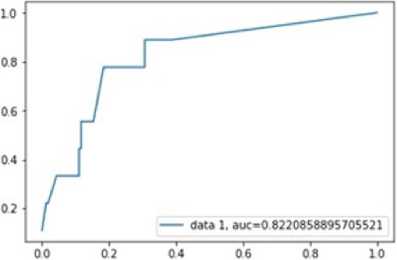
Fig.10. plot of ACU K-nearest Neighbor Classifier.

The figure shows the AUC chart and the AUC value is good which is 0.8220. This model can be used for prediction

• b)    Decision tree classifier:

  

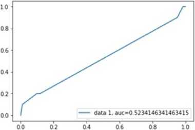
Fig.11. plot of ACU Decision tree Classifier.

The AUC value for Decision tree is 0.52. It is very less compared to K-nearest neighbor method. But this AUC value is acceptable since it is more than 0.5.

• c)    Random Forest Algorithm:

  

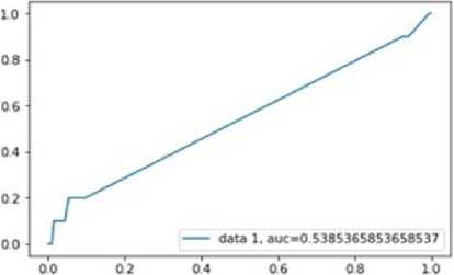
Fig.12. plot of ACU Random forest.

The AUC curve for random forest is similar as decision tree with an AUC value of 0.538536

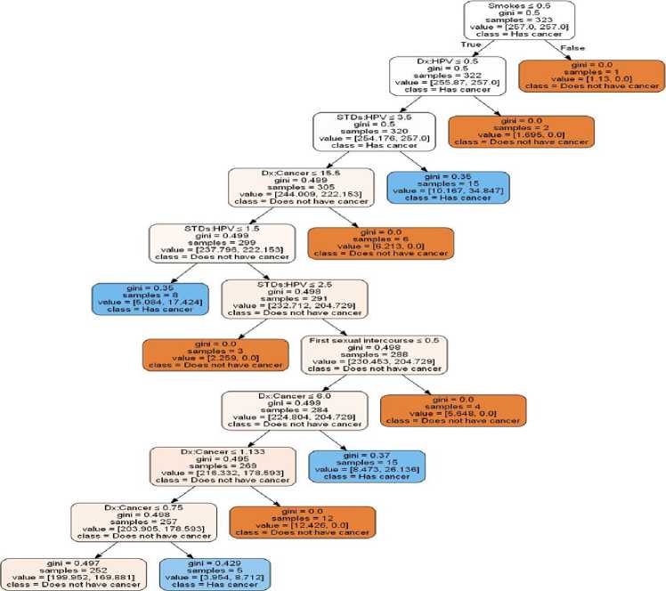
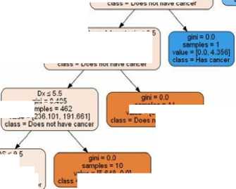
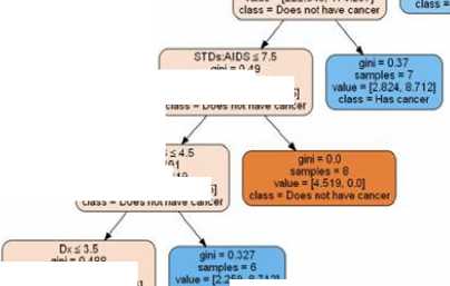
Fig.13. Random Forest tree for Prediction.

STD* moMuscum contayosum s 0 5

$ampks»514 vek* «1257.0. 257.0] class = Hai cancer

samples ■ 9 value ■ (2 259. 21.78) elate ■ Ha* cancer

DxHPV 5 0.5 gm ■ 0 499 sample* ■ 505 value-[254 741. 235 22] class ■ Does not ha.* cancer

gini ■ 0.366

samples ■ 31 value = (12 426. 39203) class ■ Has cancer

STDs Trne since first diagnosis 5 0.5 gm ■ 0 494 sample* ■ 474 value >(242 314. 196 017] class ■ Does not have cancel

yni ■ 0.495

.акте ■ (5.648. 00] ■ Does not have cancer

STDsxervkai cond/omatosis S 0.5 gm > 0.493 samples ■ 473 value = (242 314 191861] class ■ Doe* not have cancer

v*e «R

sample* >11 value >(6213. 0 0] 'have cancer

STDs AIDS S 9.5 gm = 0.496 samples ■ 452 value - [230.453. 191.661] class ■ Does not have cancer

STDs typhits 3.5 gin ■ 0493 sample* >434 value >[222 545. 174.237]

gm = 0488 sample* >413 value >[212.943. 156.814] class ■ Does not have cancer

giro ■ 0.49 samples ■ 427 value >[219 721. 165.525] class ■ Does not hM cancer

STDsAIDS gini ■ 0.491 templet «419 value = [215.202. 165 525] class ■ Does not have cancel

259,8.712] 4 class ■ Has cancer

gm • 0.429    '

samples >18 value ■ p.908. 17 424] Hat cancer

samples" 68 value ■ (33.89, 34 847] class ■ Has cancer

giro ■ 0 482 samples ■ 345 value >[179.053. 121.966] class ■ Does not have cancer

Fig.14. Decision tree Classifier tree for Prediction.

5.    Discussion

After completing the analysis, it is found that all the models are good, that is k-nearest neighbor, decision tree and random forest. K-nearest neighbor seems to be the best model with higher accuracy of the model, Higher AUC which is 0.822 as compared 0.52(Decision tree) and 0.532(random forest) which is very low. Precision recall and f1 score is also high for nearest-neighbor model. The f1 score for nearest-neighbor is 0.94 which is high when compared to decision tree (0.88) and random forest (0.90).

From the confusion matrix we can also note that false negative is zero which means that a patient with cancer will have pre- diction that he does not have cancer. It will be a bad scenario when a person having cancer will be informed that he does not have cancer. By the time symptoms starts showing it could be too late. So, it is important to choose a model that has very low false negative rates in some cases such as ours. Also, the k-nearest neighbor model has the best accuracy and AUC value which is one of the strengths of the model. So, k-nearest neighbor will be used for prediction. The dataset is biased it has a lot of zero values i.e. the patient does not have cancer for the target variable. If the dataset was little less-biased, we would have got better models and more accurate predictions. Technique used for feature selection has some disadvantages. It is difficult to know if the hill found is the highest possible hill. The local maxima are a state that is best for its neighboring states, but it might not be better than the states further away.

6.    Conclusion

• •    From the initial analysis it was clear that the data is biased

• •    In order to address the problem necessary measures were taken while modelling.

• •    Fine tuning is done on all three models to get the best accuracy.

• •    The best 3 models from each of them is selected and performance is compared

• •    It is found that all 3 models are good.

• •    But the k-nearest-neighbour model has better accuracy, precision, recall and better AUC value.

• •    The research also showed that herpes virus was able to fight cancer cells. This observation was made based on the available data and more scientific analysis needs to be carried out in order to verify this findings.