Magnetization of multilayer ferromagnetic film with a nonmagnetic interlayer

Currently, the issue we consider is of great significance because there is an international interest in multilayer magnetic systems. Such systems are used in magnetoresistive sensors, components of magnetic send-receive, spin diodes. The magnetization of a multilayer magnetic system consisting of two ferromagnetic layers with a nonmagnetic interlayer applied to antiferromagnetic substrate is considered in the presented paper. The theoretical model used for the investigation of the stated process had been introduced in paper [1]. Inhomogeneous distribution takes place in this system because of substrate influence. This is why we use a stated model.

Physical properties of the film are defined by its boundaries. A bilayer system with the ferromagnetic-on-antiferromagnetic-substrate type is investigated in research paper [1] where the boundary condition of clamped magnetization vector type had been considered.

In paper [2] it had been demonstrated that the magnetization process of such a system has a threshold type. The author [2] points out an analogue between the magnetization process and the bending of elastic rod considered in paper [3]. It is also necessary to refer to paper [4].

Later the boundary condition of the clamped vector type was replaced by condition of elastically restrained vector type by introducing an effective interlayer at the ferromagnetic-antiferromagnetic boundary [5]. In later research of bilayer ferromagnetic film, the layers of which were rigidly bond with an antiferromagnetic substrate was overlooked in [6]; using an analog of a two-part elastic shank clamped at one edge and free at the other [7].

Today the presence of a nonmagnetic interlayer in ferromagnetic systems and its influence on threshold fields and the distribution of magnetization aren’t being studied.

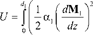
The potential energy of the magnetic system is given as expression [8]:

5Mi I 1

F\ M,l = 1a»

V    d xk ) 2

d M d M d xi dxk

a

( M ) + f ( M ² ) , (1)

where, the first summand represents the quadratic form of derivatives, w a ( M ) is the magnetic anisotropy energy, f ( M ²) is some function of M ². We only overlook isotropic ferromagnetic films where magnetization inhomogeneous is present along thickness of the object. Thereby, the second summand turns into zero and the first summand

turns into the following expression:

— a

Axis z is directed perpendicularly to the layers. A variation of the third summand results in zero because the magnetization vector length doesn’t change; therefore we shall not consider it. Thereby, the energy of the ferromagnetic layer may be represented as:

d r '

U=J

о V

—a, 21

d 1 + d s

I

M 1 H dz +

. 2 I

I - M 1 H dz ,

where d 1 , d 2 are the thicknesses, M 1 , M 2 are the magnetization densities, a 1 , a₂ are the exchange constants of first and second layers respectively; d s is the interlayer thickness, H is the applied magnetic field.

The energy of interlayer is given in the expression:

Us =-0^ M.M2, ds

where a _s is the interlayer exchange constant.

The total energy of the ferromagnetic system is:

I

- M 1 H dz +

a dz--2 M,M7

ds  ¹²

.

Angle ф 1 equals zero at the antiferromagnetic boundary because the applied magnetic field we consider is solidly joined to the antiferromagnetic anisotropy field. Where the vacuum border is angle ф ₂ shall be subject to free magnetic momentums. Mathematically, this looks like:

d 1

The value of thickness d _s is negligible in comparison to thicknesses d 1 and d 2 . It’s rather convenient to proceed to the generalized coordinates, which represent the

rotation angles between the magnetization vectors axis directed along the applied field. Then, d1 f1    J d фУ           )

U = f — a 1 M 121 — ¹ I + M 1 H cos ф 1 dz +

and x

For example let’s examine a magnetic film consisting of two ferromagnetic with equal thickness d and with a nonmagnetic interlayer:

d2 f 1 f d ф УI

+ I a₉ M 2    ²   + M^H cos ф₉ I dz -

22          22

I 2

di V           vJ

d ² ф_.    Hd ²

—r² +-- sin ф. = 0, г = 1, 2.

dz ²    a iMi    ^Yi

a,

- -^ M i M 2 cos ( ф 2 -Ф 1 ) . d_s

In these equations z is normalized variable. The solution of these equations could be represented as [1]:

d ₁

The minimum condition of potential energy gives:

5 U = a_t M ² ^1 5ф₁

^{1 1} dz ¹

2 d ф_{9 e}

+ a₂ M ₂ —- 5ф₂

^{2 2} dz ²

d i f       . d ² ф,                 I

- a_t M²— + MH sin ф 5ф₁ dz

0 V ¹¹ dz ^{2      1        1} J ¹

^d 2 f

—

^- J ^a 2 M d 1 ^V

■2 ^{d ф}                    I

₂--^2 + M^H sin ф 5ф₂ dz +

² dz ^{2        2          2} J ²

where sn( u , k ) is the Jacobi sine. Equations (11) amplified with the matching condition:

^  =a 2 M '   , dz             dz

-г УУ = С ^sin ( ф 2 ^{( 0 )-}ф 1 ^{( 1})) ,

z

and the border conditions:

M 1 M 2 sin ( ф ₂ - ф 1 ) 5 ( ф 2 - ф 1 ) d_s

= 0.

d 1

Differential equations set follows from (6) as long as variations 5ф 1 and 5ф ₂ contained in integral are arbitrary:

' d Ф2( l ) = 0

* dz

,ф 1 ( 0 ) = 0.

d2ф1.

- 1 M 1—4- + н sin ф 1 = 0, dz

_ d2 ф..

а₉ M₉--- т²- + H sin ф₉ = 0.

I 2 2 dz22

Fig. 1 represents the system of coordinates. A new coordinate system is introduced for each layer. The spiral emphasizes the interlayer interaction.

Matching of condition at point d ₁ follows from (6):

-1 d ф1 _ а s M T d1dz   ds M1

sin ( ф ₂ -ф 1 ) ,

— 1 M 1 ² d ф 1   a ₂ M 2 d ф ₂

.

d ₁ dz d ₂ dz

Here z is a normalized variable. Then we will use designation С = ( a _s M ₂)/( d _s M 1 ). This quantity characterizes the degree of the layer’s fixity. The infinitely large value of C gives ф 1 = ф ₂, substituting for first equation of (8).

The boundary conditions are also given from (6):

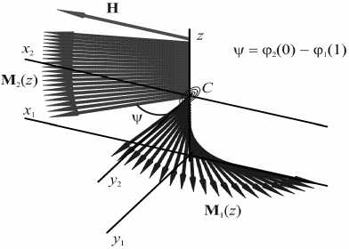
Fig. 1. Coordinate system

a_t M² d ^{ф 1} 5ф₁

^{1 1} dz ¹

d ф₂ о a₂ M ₂    ² 5ф₂

²² dz ²

= 0,

= 0.

d 1 + d ₂

Applying the border conditions and matching the condition to the solution gives:

k 1 cn u 1 = у k ₂ cn u ₂,

* p u 1 k 1 cn u 1 = ( k ₂ sn u ₂ dn u 1 - k 1 sn u 1 dn u ₂ )      (14)

( dn u 1 dn u ₂ + k 1 k ₂ sn u ₂ sn u 1 ) ,

where:

The integration gives:

п h            п M [h

M l =        , u 2 = F 2 = K ( k 2 )^{-       2}     ,

4 у hc                       4 y M 1 v hc

mx

a         a2 M->

- , Y =     22- , 0 =

I d2      4 a1 m3Cd

= 2 1 -— E ( am u 1 ) -— E ( am ( u 1 + F 2 ) ) + u i                   u i

+ E -[am F 2 , k ₂ ]

cn( u , k ), sn( u , k ), dn( u , k ) are the Jacobi cosine, sine and delta-function respectively. Constant F 1 equals zero. To define the threshold fields, elliptic modules k must be turned to zero in (14). Then, after some transformations, the transcendental equation derives from (14):

where am( u , k ) is the Jacobi amplitude (fig. 3):

п

^P 4

hr^{7 f} п hf ) 1 ^f п hf h_c ^{+ tg} I 4^ h_c I = Y c^ I 4y\ h_c

I

л

^c 7

where h^tr = H^tr/M is the threshold field. The solution of (15) relative to h^tr / h c by different values of parameters Y and p gives surface shown in fig. 2.

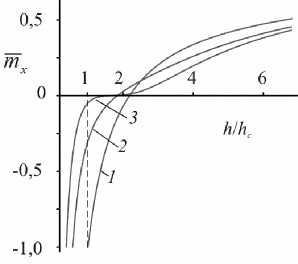
Fig. 3. The magnetization x -projection dependence on the applied field:

1 - p = 0; 2 - p = 1,4; 3 - p = 2,8

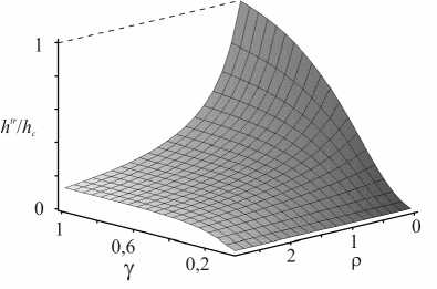
Fig. 2. Threshold field dependence on у and p

If there is no nonmagnetic interlayer ( d s = 0), and the ferromagnetic system consists of two equal layers ( y = 1), the equation (15) will depict the known expression:

, th f п i a h =             .

1 2 ) 4 d ²

In other extreme cases ( p ^ да ) the second equation of (14) gives:

п W л cos = 0,

4 hc

, th f п] a h =           .

1 2 1 d ²

This result corresponds to the ferromagnetic layer the thickness of which equals d as expected.

It’s also necessary to investigate the behavior of magnetization curves. Let’s examine a particular case where two identical ferromagnetic layers are separated by a nonmagnetic interlayer. Only variable p varies. The average value of the magnetization vector projection is presented by the following expression:

m, = J mxdz = - J cos Ф dz .

Parabola 1 corresponds to the magnetic system consisting of one ferromagnetic layer with a thickness of 2 d because p and, consequently d s equals, zero in this case. Parabolas 2 and 3 correspond to the magnetic systems involving a non-magnetic interlayer and the curve shifted to less values of the applied magnetic field at the beginning of magnetization; corresponds to a greater thickness of the interlayer.

Currently, a research on interlayer influence on threshold fields in systems of ferromagnetic-interlayerferromagnetic-antiferromagnetic types has been conducted. Also, parabolas of magnetization with different values of effective parameter p, characterizing the interlayer exchange interaction have been plotted.