MapReduce Algorithm for Single Source Shortest Path Problem

Single Source Shortest Path (SSSP) problem is to find shortest paths from the source vertex to all other vertices such that the sum of the weights of constituent edges of every path is minimized. It plays an important role in a variety of applications like Intelligent Transportation Systems (ITS) [1], Route Guidance Systems (RGS) [2], path planning in telecommunication systems, Automated Vehicle Dispatching Systems (AVDS), etc. In large networks, the shortest path is a vital problem to find betweenness centrality and closeness centrality [3, 4]. In recent years, real network graphs of transportation, social networks have grown very large. These graphs are sparse/dense, weighted/unweighted, directed/undirected in nature, have triggered to use the distributed or cloud computing environments for fast processing.

MapReduce [5], popularized by Google is a highly scalable programming paradigm capable of processing massive volumes of data in the distributed and cloud environments. It helps programmers to focus on business logic rather than various aspects of distributed computing like communication, synchronization and network failures. It has emerged as an effective and popular tool for big data processing which has automatic scalability and fault tolerance mechanism. In cloud environments, costs are estimated based on resources used. This presents an opportunity to an individual in taking decisions regarding optimal use of resources, for example, Amazon EC2 [6] charges different amount for different services like data transfer (communication), data storage, computation, rental of virtual processors etc. cloud computing provides immense independence to user to manage its resources as per computing requirements. Sometimes the user needs urgent and fast processing capability to meet its deadline also, many times users don’t bother about deadline at all. In this paper we have investigated MapReduce algorithms of SSSP that can be tuned as per the resources present in the cloud environment. A. D. Sharma et. al. [7] have highlighted the tradeoff between parallelism and communication cost in a round of MapReduce computation. More parallelism reduces the input size of every reducer, but it increases the communication cost. The communication cost of existing MapReduce algorithms of SSSP [11,12,13], discussed in section II and IV is O(E), is independent of the degree of parallelism. For one of our proposed algorithm MR-DSMR communication cost depends on the degree of parallelism and thus it exhibits the tradeoff between parallelism and communication cost also, MR-DSMR is efficient compared to all the existing algorithms.

SSSP is special problem which provides high parallelism at the cost of more work. For example, Dijkstra[8] is work efficient but doesn’t give much scope of parallelization, Bellman ford [9] is highly parallelizable but performs more work. MR-DSMR uses dsmr relaxation to reduce the work performed by the algorithm to gain the efficiency compared to BFS based algorithms

• A.    Problem Defination

Let G = (V, E) be a simple, undirected, weighted graph with non-negative edge weights. The single source shortest path problem (sssp) is computing weight vector dist(v) of a minimum weight path from a distinguished vertex s to each vertex v of the graph reachable from s.

The weight of a path is the sum of the weights of its constituent edges

• B.    Motivation & Contributions

MapReduce Algorithms of SSSP present in literature [11,12,13], are simple, offer high parallelism, uses BFS approach which requires a large number of relaxations that increases communication cost as well as number of reads/writes to HDFS. BFS based algorithms don’t give much flexibility to fully utilize memory and computing resources available on every computing node. Hence, the motivation behind research is i) To investigate an algorithm which is work efficient and ii) To devise an algorithm that can support the assignment of more/less work as required based on availability/priority of resources as well as that can efficiently utilize memory and computing resources available on every computing node in cloud environments.

We have proposed two Map Reduce algorithms of SSSP. 1) MR-DSMR, a MapReduce version of DSMR (Dijkstra Stripped Minned Relaxation) algorithm [10] and 2) MR3-BFS. We have theoretically and experimentally analyzed and compared the performance of both the algorithms with the existing algorithms present in the literature. We observed that MR-DSMR takes lesser communication and computation time compared to all existing algorithms present in the literature. Also, MR-DSMR gives us flexibility to completely utilize the available memory and processing power present in every computing node. The another proposed algorithm MR3-BFS however, takes almost equal time compared to MR2-BFS [12] but, unlike MR2-BFS, MR3-BFS doesn’t require strict constraint that all the records of a particular key must reside in the same partition in the sorted order (as per key) and each partition must reside in the same HDFS block.

The rest of the paper is organized as follows. Section II is about related works. In section III we have described proposed MR-DSMR and MR3-BFS algorithms. Section IV includes experimental results and evaluation. In section V, we have analysis and discussion and Section VI is about conclusions and related future works.

II.    Related Works

There are various parallel and distributed algorithms exist for SSSP in the literature. For our research objective existing SSSP algorithms have been studied to identify efficient algorithm that can be efficiently ported into MapReduce framework, also that can effectively utilize computing resources available at every node.

Pingali et. al. [14, 15] has classified the algorithms into ordered and unordered set. For the same problem unordered algorithms usually perform more work than their ordered counterparts, but have more parallelism due to unordered nature of processing. Dijkstra’s algorithm takes ordered approach, is less parallelizable and work efficient. In contrast, Bellman-Ford takes unordered approach, is highly parallelizable but performs more work. ∆ -stepping algorithm [16] uses a tunable parameter ∆ to get a trade-off between parallelism and work efficiency. ∆ -stepping maintains an array of buckets based of tentative distances of vertices each of size ∆ . In any iteration, parallelism is achieved by removing all the nodes simultaneously from current nonempty bucket and relaxes their light weight edges (i.e edge weights ≤ ∆ ). Heavier weight edges (edge weights ≥∆) are relaxed at the end of a phase. Chakaravarthy et. al. [17] has used hybridization of ∆ -stepping and Bellman-ford algorithm with pruning optimization to solve SSSP problem in massively parallel systems. Distributed Control algorithm [18, 19] does the relaxation at every worker node in distance order to reduce the redundant work. KLA [20] uses structure of graph to avoid redundant work. KLA asynchronously relaxes vertices which are reachable under d hops where d is a tunable parameter. DSMR [10] relaxes exactly d edges in distance order where d is a tunable parameter. Greater the value of d minimizes number of synchronizations but increases work overhead. Radius stepping [21] requires preprocessing of graph to convert the graph into a specific form and calculates radius of each of the vertex. This radius is further used to find settled vertices from the tentative list of vertices in an iteration. Crauser et.al. [22] has proposed IN/OUT criteria to parallelize Dijkstra's algorithm. They have given PRAM algorithm which uses IN/OUT criteria to identify multiple settled vertices in Dijkstra's queue whose outgoing edges can be relaxed simultaneously. G. Brodal et. al. [23, 24] has given CREW PRAM algorithm. They have proposed parallel priority data structure and used it to parallelize Dijkstra’s algorithm.

In multithreaded architecture, to achieve parallelism J. R. Crobak et. al. [25] has used Component Hierarchy [26]. Vertices inside a Component Hierarchy can be settled in any arbitrary order. Also, once component hierarchy is created it can be shared among multiple processes for computation to exploit the multithreaded architecture. M. Papaefthymiou and J. Rodrigue [27] have presented parallel Bellman-ford algorithm. Bellman-ford algorithm naturally suits parallelism because it relaxes edges of graph in any arbitrary order during any iteration. The algorithm presented by authors in [28] uses graph partitioning approach for parallelization. The Algorithm partitions the graph into disjoint sub-graphs, assigns each sub-graph to a processor. In the first iteration only one processor, which has source node information, computes temporary shortest path. Next, boundary information is exchanged between adjacent sub-graphs. The process continues until there is a state of no message exchange between the adjacent sub-graphs, occurs.

• A. Related works(MapReduce \Algorithms)

MapReduce [5] is a popular programming framework for large data processing. It is based on key value data model. It offers fault tolerant, scalable processing in distributed and cloud environments. It gives freedom to programmer to focus on business logic rather than various aspects of distributed computing like communication, synchronization and network failures. A

MR-BFS : J. Lin and C. Dyer [9] have presented MapReduce algorithm for SSSP (Algorithm 1). In map phase the algorithm emits graph data structure as well as distances of all those vertices which are adjacent to currently active vertices (line 8 and 6). In reduce phase, the algorithm selects minimum tentative distance and updates the status of vertex (line 11, 12, 14). At line 15 MR-BFS emits graph data structure along with the distance and status of each of the vertices. The algorithm requires graph data structure to be maintained throughout of iterations. This increases the communication cost as well as number of reads/writes cost to HDFS in every iteration

Schimmy-BFS: Lin and Schatz [13] proposed schimmy design pattern for graph algorithms. Shimmy design uses parallel merge join between graph and messages in reduce phase to avoid shuffling of large graph. However, it requires graph data structure to be written to HDFS between iterations. Thus schimmy design pattern doesn’t reduce HDFS writes cost. However, it significantly reduces communication cost

MR2-BFS : Kajdanowicz et. al. [12] has proposed MR2-BFS. MR2-BFS is based on Map Side join. The algorithm joins messages and graph data structure in Map phase. Map Side join is efficient compared to Reduce side join (Schimmy-BFS) as it avoids the need of writing graph data structure to HDFS between iterations. Thus MR2-BFS significantly reduces communication cost as well as number of HDFS writes. However, the algorithm requires all the records of a particular key must reside in the same partition in the sorted order (as per key). Also, each partition must reside in the same HDFS block. These strict constraints require pre-processing of the graph.

All the mapreduce algorithms of SSSP discussed above uses BFS approach. They all require same number of relaxations. However, they are different in terms of utilization of map reduce frame work to reduce HDFS writes and data shuffling cost.

For a good mapreduce algorithm wall clock time is a significant factor [30]. A wall clock time is the actual amount of time to perform a job. For an iterative MapReduce algorithm following parameters affect the total wall-clock time 1) Communication cost 2) Number of read and write to HDFS 3) Computation cost of a

Reducer and 4) Computation cost of a Mapper.

More parallelism decreases the wall clock time, increases the communication cost, high communication cost ultimately increases the wall clock time and naturalizes the benefit gain through high parallelism. Ullaman[30] has included computation cost of mapper to communication cost as communication cost depends on the key-value pair generated by mapper. A.D. Sharma et. al. [7], Ullaman [30], have discussed communication cost depends on replication rate (rate at which number of keyvalue pairs generated per input element), and computation cost of a reducer depends on reducer size (input size of each of the reducer). Higher replication rate increases the parallelism and communication but decreases the reducer size. Thus, replication rate and reducer size heavily affect the wall clock time of a mapreduce algorithm. For BFS based algorithms, replication rate of an input to mapper is degree of vertex (v a ) where v a is an active vertex, and reducer size is also the-degree of vertex v a . Thus for BFS based algorithms, replication rate and reducer size both depends on the nature of the graph. One of our proposed algorithm MR3-BFS uses BFS approach with reduce side join. BFS approach uses chaotic relaxation which is inefficient in terms of total work done by any SSSP algorithm. Another proposed algorithm (MR-DSMR) is work efficient compared to BFS as it uses DSMR relaxations.

Algorithm 1: MR-BFS

• 1:    class Mapper

• 2:   method Map(nid n, node N)

• 3:      d ^ N.Distance

• 4:        if (N.Active=True)

• 5:            for all nodeid m ∈ N.AdjacencyList do

• 6:               Emit(nid m, d+w(nm))

• 7:           N.Active=False

• 8:       Emit(nid n, N)

• 1:    class Reducer

• 2:  method Reduce(nid m, [d1,d2,])

• 3:       dmin ^ infinity

• 4:      M ^ null

• 5:        for all d ∈ [d1,d2,...]

• 6:            if IsNode(d) then

• 7:M

• 8:            else if d < dmin then

• 9:             dmin ^ d

• 10:       if (M = null or M.distance > dmin) then

• 11:          M.distance ^ dmin

• 12:          M.active ^ True

• 13:       else

• 14:          M.active ^ false

• 15:     Emit(nid m, node M)

III.    Proposedworks

• A.    MR3-BFS

MR2-BFS [12] requires all the records of a particular key must reside in the same partition in the sorted order

(as per key). Also, each partition must reside in the same HDFS block. Thus MR2-BFS requires preprocessing of graph. Our proposed algorithm MR3-BFS also requires preprocessing to partition the graph. However, it doesn’t require a partition must reside in the same HDFS block.

The distributor of MR3-BFS is a mapreduce job which runs for a single round. It partitions the graph in to exactly r disjoint subsets v 1 , v 2 , v3  v r such that all these subsets represent subgraphs obtained from vertices present in v z plus all the adjacent edges of vertices present in v z. Vertex idof a vertex v is the key and value is the edges adjacent to the vertex v. The distributor creates exactly r files one for each partition sorted as per key. The partitioner of distributer and MR3-BFS both must be the same function. For our implementation the partitioner partitions vertices using mod operation i.e. vertex_id%r (here r is the number of reducers).

The algorithm MR3-BFS is presented in Algorithm 2. In Reduce phase MR3-BFS reads its partitioned graph (at line 6), and computes the distances of adjacent vertices of active vertices (at line 16, 17). mapper simply forwards messages (distance and status) of a vertex to the partitioner (line 3). After shuffle and sort each messages reach to reducer. Next, the reducer selects new minimum tentative distance and new status of the vertex (At line 10 to14). If status of the vertex is active then distances of adjacent vertices are calculated and emitted with status A (active) (line 15-17). Once all the adjacent edges of the vertex are relaxed the vertex itself is emitted with status “R” (line 19). A vertex which is received from mapper with status “R” is emitted immediately as its all adjacent edges are already relaxed in the previous iteration. (line 21).

Algorithm 2: MR3-BFS

• 1:    class Mapper

• 2:    method Map(id n, [distance,status]))

• 3:        Emit(id n, [distance,status])

• 1:    class Reducer

• 2:    method Initialize

• 3:       P.OpenGraphPartition()

• 4:    method Reduce(id n,[p1,p2,p3......])

• 5:        repeat

• 6:           (id n, vertex N) ^ P.Read()

• 7:       until n=m

• 8:       dmin ^ infinity

• 9:       status ^ ""

• 10:       for all p belongs to [p1,p2,p3....] do

• 11:           [new_distance,new_status] <- p.split()

• 12:          if(dmin > new_distance)

• 13:              dmin ^ new_distance

• 14:               status ^ new_status

• 15:       if (status="A")

• 16:           for all nodeid m ∈ N.AdjacencyList do

• 17:              Emit(m,[dmin+w(nm),”A]”)

• 18:               counter++

• 19:          Emit(n,[dmin,”R”])

• 20:       else

• 21:           Emit(n,[dmin,status])

The iteration of mapreduce job continues until there is the state that no more active vertices present in any of the reducers. The Driver program detects any active vertices present in any of the reducers. In hadoop, it is achieved through counter variable which gets incremented if any active vertex is present (line 18 of reducer).

Comparison between MR2-BFS and MR3-BFS : MR2-BFS and MR3-BFS both perform chaotic relaxations. Both the algorithms require preprocessing of graph. Also, both the algorithms don't require shuffling and HDFS write of large graph through out of iterations. The total communication cost of both the algorithms is O(E) because both the algorithms perform chaotic relaxations. Time and Space complexity of any reducer of MR2-BFS & MR3-BFS is O(deg(v)). The time complexity of a mapper of MR2-BFS is O(deg(v).k) where k is the number of records in a HDFS block. Time complexity of a mapper of MR3-BFS is O(k) as it simply emits vertex its distance and status record by record. Thus, efficiency wise MR2-BFS and MR3-BFS both are almost same.

MR2-BFS is based on map-side join which requires all the records of a particular key must reside in the same partition in the sorted order (as per key) and each partition must reside in the same HDFS block. In contrast, MR3-BFS doesn’t require all the records of a particular key must reside in the same HDFS block. This is the advantage of MR3-BFS over MR2-BFS.

• B.    Overview of DSMR Algorithm

DSMR algorithm [31][10] runs into multiple supersteps. each supersteps consists of three stages. 1) Each processor applies Dijkstra's algorithm to its assigned subgraph, relaxes vertices in distance order until exactly D edges are relaxed. Edges whose destination vertex are present locally in the processor's memory is relaxed immediately, the destination vertices which are not present locally are buffered. 2) After D edge relaxations the algorithm enters into communication phase and does all-to-all communication to exchange the buffered relaxations. 3) Each processor maintains a set of active vertices (vertices whose distance is updated and whose all edges are yet to be relaxed). The supersteps continue until there is a state that no more active vertices present in any of the processor.

The distributor of DSMR algorithm partitions the vertices of graph into K (No. of processors) disjoint subsets V 1 , V 2 , V3 V k , using these K subsets K subgraphs are obtained from vertices in the partition V z plus all adjacent edges of vertices present V z.

• C.    Overview of Proposed MR-DSMR algorithm

The proposed Map Reduce algorithm (we refer this algorithm as MR-DSMR) is the Map Reduce implementation of DSMR algorithm. The distributor of MR-DSMR partitions the vertices of graph into r disjoint subsetsV 1 ,V 2 ,V3 V r using these r subsets r subgraphs obtained from vertices in the partition V z plus all adjacent edges of vertices present in V z. The mapper of distributor assigns a unique key to each of these partitions.

After shuffle and sort a partition is assigned to a reducer (based on key generated by mapper). A Reducer is the owner of all the vertices present in a partition. A Reducer is responsible to find/maintain the distances of the vertices present in its assigned partition. “Fig. 1” shows a sample assignment of subgraph to each of the reducers. here vertices are partitioned into three disjoint subsets S1={v 1 ,v 4 ,v 7 }, S2={v 2 ,v 5 ,v 8 }, S0={v 3 ,v 6 ,v 9 } using distributor logic of mapper as vertex_id % no. of reducers. The subgraph obtained by vertices of set S1 with their adjacent edges is assigned to Reducer1. Similary subgraph obtained by vertices of partition S2 is assigned to Reducer2 and subgraph obtained by vertices of partition S3 is assigned to Reducer 0.

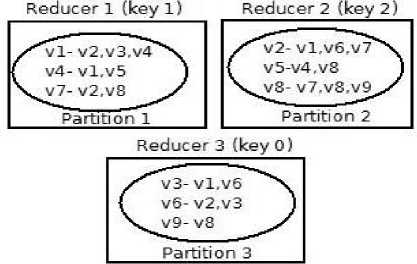
Fig.1. A sample assignment of Sub graphs to Reducers

The Map-Reduce job of distributor is non-iterative in nature, runs for at most two rounds, creates subgraph for each of the reducer. Next, the reducer of MR-DSMR reads its assigned subgraph, applies DSMR algorithm and emit buffered distances. The mapper of next iteration diverts buffered distances to reducers. This process continues until there is a state that no active vertices present in any of the reducers. The algorithm MR-DSMR is discussed in details in sub section 3.5.

• D.    Partitioning of Graph (The Distributor of MR-DSMR)

Data Skew and work balance among processing nodes are the major concern of a distributed algorithm. Skew in data heavily affects the work assignment to every processing node. A good graph partitioning algorithm is required to partition the graph to get the optimal performance. Chakaravarthy et. al. [17] has used vertex splitting technique and intra node balancing strategy to partition the graph. Maleki et. al. [10] has also used vertex splitting technique for high degree vertices and randomly suffling of low degree vertices to each of the processing nodes. The distributor of MR-DSMR is a Map Reduce Job which runs for at most two rounds of iterations. Our Partitioning algorithm uses similar concept as presented in [10].

To partition the vertices of the graph, Mapper emits specific key of a partition which is further grouped by reducer. There can be various partitioning approach. But, for our implementation, we have used random partitioning using mod operation. The Mapper of Distributor accepts adjacency list of graph as input, does random partitioning of vertices using mod operation.

Mapper emits key as vertex_id % r (here r is the number of reducers) and value as vertex_id along with its adjacency list. For high degree vertices (which have degree greater than a threshold value), the mapper creates exactly r proxies (one for each of the reducers), and assigns 1/rth number of adjacent edges of original vertex to each of the proxies. Further, mapper emits keys in such a way that each of the proxies should go to each of the reducers. Each of These r proxies are connected to the original vertex with weight 0. Reducers receive the subgraphs with the specific key and create exactly r files one for each of the subgraph. A sample assignment of subgraph is shown in “Fig. 1”.

The Shuffling of low degree vertices is done during reduce phase. A reducer counts number of edges in its assigned subgraph. if number of edges, it receives from mapper with in a specific range (90%-110% of E/r where E is total edges of graph, For very large graph (95-105)%of E/r) it doesn't do the shuffling otherwise The reducer which receives more than 110% of E/r edges identifies low degree vertices and groups into exactly r groups (one group for each of the reducers) in such a way that each group should have almost same number of edges. Next, reducer keeps a group for itself and creates proxies for each vertex of those groups which are marked for other reducer. A proxy is connected to all the adjacent edges of the vertex, and a vertex is connected to its proxy with weight 0. The generation of proxy number requires special care as keys are assigned using mod operation. The grouping of low degree vertices requires extra care to achieve assignment of almost equal number of number of edges for each of the reducers.

The Distributor requires at most two iteration of MAP Reduce job. However, a distributor of MR-DSMR can also be a sequential algorithm.

The primary objective of distributor is: 1) the distributor should partition the vertices of a graph in such a way that each partition should have a separate key 2) Every partitions should have almost equal number of edges 3) Random partitioning doesn't utilize the property of the graph. Random partitioning can be replaced with some other partitioning strategy that can utilize the property of the graph to achieve significant performance gain.

• E.    Relaxation

Relaxation is a basic operation of SSSP. Relaxation always keeps optimal solution and discards non-optimal one. Successive relaxation results to successive approximation to the most optimal solution. Relaxation operation generates new distance of destination vertex which may present in a partition or which belongs to other partition. Given an edge e = (u,v) the operation Relax(u,v) is defined as

Relax(u,v) -> min(d(v),d(u)+w(u,v)). Here d(v) is old distance of v. d(u)+w(u,v) is the new distance of vertex v from the source vertex.

• F.    MR-DSMR

Mapper: Each Mapper Reads the buffered distances from Hdfs. For the first iteration source vertex with its distance is buffered. Hence, input file of first iteration contains s 0 (where s is the source vertex and zero 0 is its distance). For all subsequent iterations buffered distances are written to HDFS by reducer of the previous iteration. The algorithm MR-DSMR is shown in Algorithm 3. The mapper of MR-DSMR simply diverts the vertices with its buffered distances to reducer (at line 5). At line 3 an array track is used to ensure that in every iteration mapper should emit the key of all the partitions. (line 7-9).

Reducer : Each Reducer writes the distance file to HDFS. A distance file contains node_id(v), its distance(d(v)) and status(st(v)) of every discovered vertex v. There are two types of vertices present in the distance file. A vertex with status "a" represents active vertex, a vertex with status "r" represents relaxed vertex. Active vertices are those vertices whose adjacent edges are yet to be relaxed. Relaxed vertices are those vertices whose adjacent edges are relaxed. For the first iteration the distance file doesn't exit. For the subsequent iterations each reducer reads distance file, creates a data structure A of active vertices, creates a data structure R of relaxed vertices and updates partial state variables (at line 3). Reducer receives the buffered distances from mapper and updates A and R (line 4 to 6). Reducer creates work list (wl) of active vertices (at line 7). Reducer reads its own paritioned subgraph and keeps in a suitable data structure (line 8). Next, Reducer calls DSMR algorithm for relaxation of vertices in distance order (line 9). A vertex whose all the adjacent edges are relaxed is removed from A and added into R (line 17-19, 28-30 of function Relaxvertex()). Newly discovered vertices, if it belongs to reducers' own partition are added into A immediately otherwise, it is emitted with its distance. Exactly after D relaxations, relaxation process is aborted partial state (consists of node_id (pv), its distance (d(pv)), and index of the graph where relaxation aborted (st(pv)) is updated which is further written to distance file along with R and A (line 10). For our implementation we have used priority queue for implementation of work list of active vertices. However, it can be replaced with any other efficient implementation as it is suggested in [10].

Algorithm 3: MR-DSMR

• 1:    class Mapper

• 2:   method (v, d(v))

• 3:       track[r] = new boolean array[r];

• 4:        track[r] ^ false;

• 5:        emit(v%r, [v,d(v)])

• 6:       track[v%r]^true;

• 7:       for each of (t ^ 0;t < r; t++)

• 8:              if(track[t]=false)

• 9:                emit(t,”dummy”);

1: class Reducer

• 2:    method Reduce(key,[(v₁,d(v₁)), (v₂,d(v₂))^])

• 3:       Read the distance file from HDFS, Create data

structure A of active vertices, create data structure R of relaxed vertices and update partial_vertex, partial_distance and partial_index variables.

• 4:         For all (v,d(v)) e [(v i ,d(v i )), ,(v 2 ,d(v 2 ))^] do

{

• 5:                  [v,d(v)J^ (v.d(v)).split()

• 6:                 Adjust_distances(v, d(v)) // optimal

distance retained

8                     }

• 7:        create worklist (wl) of active vertices using data

structure A.

• 8:      Read owned partitioned subgraph from HDFS

and keep it into a suitable data structure.

• 9:       void Dsmr()

• 10:      write_distance()

• 1:    void Adjust_distances (vertex v, d(v))

• 2:    if (v ∉ to R.v)

• 3:         if (v ∉ A.v)

• 4: .            insert [v,d(v)] into A

• 5:         else

• 6:              if (d(v) < A.d(v))

• 7:                A.d(v) ^ d(v)

• 8:    else

• 9:         if (R.d(v) > d(v))

• 10:          remove [v,d(v)] from R.

• 11:           insert [v,d(v)] into A.

1:void Dsmr()

• 2:    do {

• 3        Int m = min i: !IsEmpty(wl[i]);

• 4:       while (!IsEmpty(wl[m]) && relaxed

• 5          {

• 6:             if ((vertex v=wl[m].pop())=partial_vertex)

• 7:                 RelaxVertex(v,min,partial_index)

• 8:               else

• 9:                RelaxVertex(v,min,0)

• 10       }

• 11: } while (m < infinity || relaxed < D)

• 1:    Relaxvertex (vertex v, int d(v),int i)

• 2:  boolean flag=true

• 3:     if (i=0)

• 4:       For each Edge vu in edges(v) do

• 5:           relaxed++

• 6:            i++

• 7:            if (u%r=key)

• 8:                RelaxEdge(u,d(v)+w(vu))

• 9:               else

• 10:               emit(u,d(v)+w(vu))

• 11:           if (relaxed >=D)

• 12:            pv ^ v

• 13:               d(pv)^ d(v)

• 14:                st(pv)^ i

• 15:                 flag^false;

• 16:                break ;

• 17:        if (flag)

• 18:           erase (v,d(v)) from A

• 19:           Insert (v,d(v)) into R

• 20:    else

• 21:       For each Edge vu in edges(v) starting from

index i to degree(v) do

22:	relaxed++
23:	i++
24:	if (u%r_no=key)
25:	RelaxEdge(u,d(v)+w(vu))
26	else
27:	emit(u,d(v)+w(vu))
23:	if (relaxed >=D)
24:	pv ^ v
25:	d(pv) ^ d(v)
26:	st(pv) ^ i
27:	break ;
28:	if (flag)
29:	erase (v,d(v)) from A
30:	Insert (v,d(v)) into R

• 1:    RelaxEdge (Vertex u, int newDist)

• 2:   if (u ∉ A.node_id && u ∉ R.node_id)

• 3:        insert(u,d(u)) into A

• 4:        wl[d(u)].insert(u)

• 6:       iteration counter++

• 7:   else if ((u ∉ A.node_id && u ∈ R.node_id))

• 8:        if (newDist < R.d(u))

• 9:            erase(u,d(u)) from R

• 10:          d(u) ^ newDist

• 11:           insert(u,d(u)) into A

• 12:           wl[d(u)].insert(u)

• 13:           iteration counter++

• 14:    else

• 15       if (u ∈ A.node_id && u ∉ R.node_id)

• 16:           if(newDist < A.d(u))

• 17:                wl[d(u)].erase(u)

• 18:              A.d(u) ^newDist

• 19:                wl[d(u)].insert(u)

• 20:               iteration counter++

• 1:    write_distance()

• 2:  create file in HDFS with iteration_no and key

embedded into the file name.

• 3:        For each entry [v,d(v)] of A do

• 4:             write(v,d(v),"a")

• 5:        For each entry [v,d(v)] of R do

• 6:             write(v,d(v),"r")

• 7:        write(-1, p(v), d(p(v)), st()) // -1 is an indication

of partial variable

The mapreduce iteration of MR-DSMR continues until there is the state that no active vertices present in any of the reducer. Driver program using counter variable (at line 6, 13, 20 of function Relaxedge()) detects the presence of active vertices.

IV. Experimental Results and Evaluation

A small Hadoop cluster of 9-nodes is set up to evaluate all the presented algorithms. One node is configured as master and eight nodes are configured as slaves. Each of these nodes has 4 GB of RAM and 256 GB hard drive. All the nodes are connected with 100 Mbps Ethernet network. Experiments are conducted on Hadoop version-1.2.1 and JAVA JDK version “1.8.005”. All the algorithms are tested with RMAT graphs [32] with different scales. Graphs are generated with SSCA #2 [33]. Graph 500 type-2 benchmark setup (a=55, b=c=.1 and d=.25) with edge factor 16. Edge weights are chosen uniformly random from [1…256]. Best D value for lowest execution time of MR-DSMR is searched from {29, 210, …..224}. We have evaluated our proposed algorithms with MR-BFS on different graph scales. MR2-BFS is theoretically evaluated and compared with MR3-BFS in section 3.1.

Data presented in “Fig 2”, “Fig.3”, “Fig4” are captured using Hadoop counters. Hadoop MapReduce framework provides counters to capture job statistics of a mapreduce job. Counters related to HDFS read, HDFS write, data shuffled between mappers and reducers are captured for each iteration (i.e for each MapReduce job) which is further summed up and percentage is calculated with respect to input graph size. The wall clock time, presented in “Fig 5”, “Fig 6”, “Fig 7” is the time duration of job submission and completion

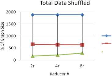
Communication Cost : “Fig. 2” shows total data shuffled across the network (in % of the original input graph size) of MR-BFS, MR3-BFS and MR-DSMR algorithms tested on RMAT (scale 20) graph. It is evident from the figure that MR-DSMR is efficient in terms of communication cost compared to all other algorithms. The communication cost of MR-BFS is high as it has to shuffle graph data structure as well as adjacent edges of active vertices through out of iterations. The communication cost of other BFS based algorithms like schimmy-BFS, MR2-BFS, MR3-BFS is O(E) i.e. the number of edges present in the graph. For the algorithm MR-DSMR the communication cost depends on buffered distances. Higher the buffered distances higher the communication cost. Thus, increasing the degree of parallelism doesn’t affects the communication cost of all the BFS based algorithms whereas, for MR-DSMR it varies with the varying number of reducers as it evident in the Fig.2.

MR-BFS

—*-MR-DSMR

Fig.2. Total data shuffled across the network of MR-BFS, MR3-BFS and MR-DSMR for varying numbers of reducer.

—e-MR3-BFS

HDFS Read: Increase in number of HDFS reads/writes indirectly increases the communication cost. “Fig. 3” shows total number of HDFS read (in % of original input size of the graph) for varying number of reducers of all the algorithms. It is evident from the figure that compared to MR3-BFS and MR-DSMR, MR-BFS requires less number of HDFS read as MR-BFS doesn’t write adjacent edges of active vertices to HDFS between iterations.

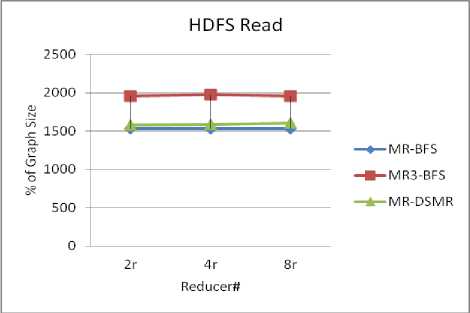
Fig.3. Total number of HDFS read of MR-BFS, MR3-BFS and MR-DSMR for varying number of reducers.

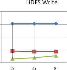
HDFS Write : MR3-BFS and MR-DSMR don’t write graph data structure to HDFS between iterations whereas, MR-BFS writes graph data structure through out of iterations. “Fig.4” shows number of HDFS writes (in % of original graph size) for MR3-BFS and MR-BFS. It is evident from the figure that MR-DSMR requires less number of HDFS write compared to MR3-BFS and MR-BFS. Also, HDFS write doesn’t vary for the BFS with the varying number of reducers. But, it varies for MR-DSMR. Thus, degree of parallelism affects HDFS write of MR-DSMR.

У 1500

2 1000

О

S 500

Reducers #

• Fig.4. Total number of HDFS writes of MR-BFS, MR3-BFS and MR-DSMR for varying number of reducers.

Total Wall-clock Time : “Fig. 5” shows wall clock time of MR-BFS, MR3-BFS and MR-DSMR algorithms of RMAT scale-20 graph. MR-DSMR requires less number of relaxations (less work) compared to MR-BFS and MR3-BFS. Hence, it is efficient compared to BFS based algorithms. MR3-BFS is efficient compared to MR-BFS due to less number of HDFS write and due to less communications. “Fig. 7” shows wall clock time of all the algorithms on RMAT (scale 22) graph (1 GB data set). It is evident that MR-DSMR is efficient compared to MR-BFS and MR3-BFS.

Scalability : All the algorithms are examined with varied graph sizes on varied number of computing nodes. “Fig.

5” shows total time taken by MR-BFS, MR3-BFS and MR-DSMR to compute sssp on Rmat (scale 20) graph for varying number of reducers. For All the algorithms it is evident that total elapsed time decreases with the increase in number of reducers.

Weak scaling is also examined by increasing the graph size with the increase in number of reducers “Fig. 6”. One interesting observation is that all the three algorithm behavior is almost same for varying number of reducers. For 2 to 4 reducers there is increase in execution time there after linear scaling results are obtained. This may be due to the input graph and random generation of edge weights.

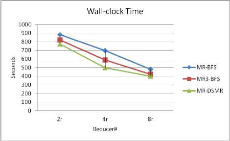
Fig.5. Total Wall-clock Time of RMAT20 graph of MR-BFS, MR3-BFS and MR-DSMR algorithms for varying number of reducers.

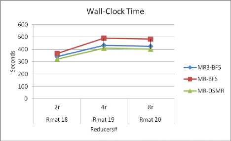
Fig.6. Wall clock time of MR-BFS, MR3-BFS and MR-DSMR for varying graph size and varying number of reducers.

Computation time and space requirement of BFS : The maximum computation time required for any of mapper/reducer of BFS based algorithms is O(deg(v)) where deg(v) is degree of any vertex v. The space requirement of any of mapper/reducer is also O(deg(v)). Thus, cpu cost as well as memory cost of any reducer or mapper of BFS doesn’t get affected with increasing or decreasing the number of reducers.

Computation time and space requirement of MR-DSMR: Suppose Vp and Ep is the number of vertices and edges present in the subgraph obtained after partition. If we consider the worst case scenario, the total number of buffered distances received by any of the reducer is O(Vp). Also, in worst case, the size of A and R together is not more than Vp. Hence, CPU Time required to read the graph and keep in memory is O(Vp + Ep), Time required to read the distance file is O(Vp), Time required to run DSMR for our implementation (using priority queue) is O((Vp + Ep)log Vp). So, total time complexity of any of the reducer in any iteration is O((Vp + Ep)log Vp) (in worst case). In fact, in any iteration there are many vertices which are get settled also, there are some vertices which are already relaxed in previous iteration. So, they never go to the work list of active vertices. Hence, in normal scenario Va (number of active vertices) is far less then Vp. Also, in any iteration at most D relaxations are allowed. Thus, in normal scenario total execution time of any reducer of MR-DSMR is far less then O((Vp + Ep)log Vp). DSMR implementation can be replaced with any other implementation like Fibonacci Heaps or the implementation presented in [10] for better efficiency.

The space requirement for any of the reducer of MR-DSMR is O(V p + E p ) . Thus time complexity and space complexity of any reducer of MR-DSMR depends on the partial vertices and edges assigned to a reducer. So, increasing or decreasing the number of reducers i.e. degree of parallelism affects the time and the space requirement of a reducer of MR-DSMR.

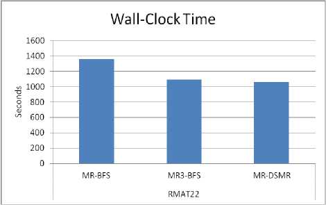
Fig.7. Total Elapsed time of Rmat22 graph of MR-BFS, MR3-BFS and MR-DSMR algorithms on 8 reducers.

Wall clock time of a job is the time duration during which computing resources held by a computing system. For a MapReduce job, total wall clock captures almost all the parameters of MapReduce computation like parallelism, execution time of Mappers/Reducers, data shuffled across computing resources and number of reads/writes to HDFS. In previous section we have observed that for BFS based algorithms data shuffled across networks, number of HDFS reads/writes, time/space requirements of a mapper/reducer don’t get affected with the degree of parallelism. In contrast, all these parameters get affected with the increase and decrease of degree of parallelism for MR-DSMR. BFS and MR-DSMR both assign more and less work to every computing node as per the degree of parallelism i.e. higher degree of parallelism lead to assignment of less amount of work to every computing node. However, BFS doesn’t completely utilize available memory and computing power available on every processing nodes as time and space requirement of any mapper/reducer is O(dev(v)) which is independent of degree of parallelism. MR-DSMR gives us opportunity to utilize memory and computing power available in every node processing node by changing the degree of parallelism.

All the BFS based algorithms as well as MR-DSMR assigns less/more work to every processing node depending on the number of computing nodes. This makes all the algorithms scalable with the resources. However, as discussed, BFS based algorithms don’t give much freedom to completely utilize memory and computing resources available in every computing nodes. MR-DSMR gives us freedom to utilize memory and computing resources available in every processing node by changing the degree of parallelism. Hence, MR-DSMR gives us freedom to use the resources available in cloud environments. For example, for Amazon EC2 cloud, a 10-node cluster running for 10 hours costs the same as a 100-node cluster running for 1 hour. Hence, for any algorithm, to minimize the cost and time associated with the processing, it is better to fully utilize available memory and computing power of every processing node. Thus, MR-DSMR fits well in cloud environment compared to BFS based algorithms. Also, MR-DSMR is efficient compared to BFS based algorithms.

VI.    Conclusion and Future Works