Mathematical Model of Delivery Speed in DevOps: Analysis, Calibration, and Educational Testing

DevOps is considered an interdisciplinary concept that integrates development and operational processes and aims to accelerate software delivery, improve product quality, and ensure service stability [1 –3]. In the context of digital transformation, DevOps has become a key factor in organizational competitiveness. A growing body of research confirms this. These studies address the technical, organizational, and cultural aspects of implementing DevOps [4-9].

The scientific literature emphasizes that DevOps goes beyond a simple instrumental approach and establishes a new model for managing the software lifecycle. Works [10-12] emphasize the strategic role of DevOps. In particular, these works focus on reducing the development cycle, improving communication, and fostering a culture of cooperation among teams. Studies [7, 13] demonstrate that implementing DevOps increases IT team productivity and improves user satisfaction. However, several studies [14, 15] highlight the challenges associated with this approach, including resistance to change, a lack of necessary skills, and the complexity of integrating automation and processes.

Despite significant progress in DevOps research, most studies remain focused on qualitative aspects, including practice descriptions, critical success factor analyses, cultural transformations, and metrics classifications. Few studies address process formalization and provide quantitative models that describe parameter interactions, including development speed, automation level, CI/CD maturity, architectural complexity, and system stability, capable of predicting their impact on performance indicators.

The lack of a mathematical basis complicates comparisons of DevOps practices and prevents an objective assessment of their effectiveness, hindering the development of universal recommendations for organizations of different sizes. Therefore, formalized models are needed to quantitatively describe DevOps system behavior while accounting for nonlinear and threshold effects, enabling scenario analysis and calibration using practical or training data.

The S delivery speed model proposed in the article accomplishes these tasks. It integrates the technical, operational, and architectural parameters of DevOps into a single mathematical structure. This enables analysis of processes and prediction of results related to CI/CD, automation, and system complexity.

2.    Literature Review

A review of the current literature reveals that DevOps is considered a multidimensional socio-technical phenomenon. This approach centers on performance metrics, critical success factors, a culture of collaboration, and the integration of technical practices. The DevOps literature systematizes these components in various research areas, with most works emphasizing similar trends. These include the importance of automation, stability, process transparency, and interaction between teams. However, the literature rarely considers their quantitative and formalized representation.

Article [16] offers the most comprehensive systematization of DevOps metrics. These include Mean Time to Recovery (MTTR), Deployment Frequency, Change Lead Time, and Change Failure Rate. The authors categorize these metrics into productivity, quality, and stability, emphasizing their role in data-driven decision-making. However, despite its detailed classification, the work does not consider the mathematical relationships between metrics. It also does not offer models capable of predicting changes in DevOps process productivity.

Studies [8, 17, 18] analyze critical success factors (CSFs) of DevOps and highlight technical, organizational, and sociocultural dimensions. Despite different contexts, the authors draw similar conclusions: a combination of modern automation tools, effective architecture, strategic management support, team interaction, and a culture of collaboration determines DevOps success.

Paper [19] emphasizes the importance of leadership, automation, and cross-team collaboration. The study reveals that DevOps results in greater stability and shorter development lifecycles. However, the authors provide only qualitative indicators of the impact of these factors. A similar approach is presented in [20], where the authors represent DevOps using a Venn diagram. The diagram illustrates the intersection of development, operations, and management. The authors emphasize the structural interdependence of DevOps components. Nevertheless, they do not introduce formal or stochastic models to describe these interactions.

A review of the literature reveals several important trends, as a significant number of studies have examined DevOps metrics [16], critical success factors [8, 17, 18], and organizational and cultural factors of DevOps [19, 20], with most approaches based on qualitative classifications or empirical observations. Virtually no models quantitatively formalize the interaction between the technical, organizational, and architectural factors of DevOps.

Thus, despite the large number of available studies, there is a lack of formal, mathematical models capable of describing the dynamics and interdependence of key DevOps parameters. The S delivery speed model proposed in this article incorporates ideas from the aforementioned studies. It presents these ideas in the form of functional dependencies. The model also allows for impact analysis, scenario modeling, and data calibration.

3.    Methodology

This study combines a systematic analysis of DevOps processes, formal mathematical modeling, and model testing using pseudo-real and training empirical data and consists of four interrelated stages. The first stage involves conceptualizing key DevOps parameters. The second stage involves forming the analytical structure of the model. The third stage involves calibration and initial verification. The fourth stage involves training, testing, and interpreting the results.

Based on the literature review, we identified five key parameters that significantly impact software delivery speed and represent modern DevOps practices. D denotes development speed. A reflects the level of process automation. CI/CD describes the maturity of the continuous integration and delivery pipeline. R shows the availability of resources, including human and infrastructure resources. C characterizes the system's architectural complexity.

We selected these variables based on their presence in empirical DevOps frameworks, such as DORA, SPACE, and the Accelerate framework. Numerous studies have confirmed their impact on team productivity.

During the second stage, we identified functional dependencies among parameters, focusing on several aspects. First, we examined nonlinear effects, including saturation, thresholds, and the diminishing marginal utility of automation. The second is the synergistic interaction between A and CI/CD. The third aspect was the negative exponential impact of CI/CD complexity on the delivery process, while the fourth aspect concerned parameter elasticity, which reflects the relative strength of impact.

This stage laid the groundwork for developing the S-delivery speed model. We present it in the next section.

The study used a pseudo-realistic dataset of 20 observations to quantify the parameters, which replicated typical DevOps conditions described in the DORA and Accelerate reports. The data included the values of D, A, CI/CD, R, and C, as well as the observed S values.

Calibration was performed using the least squares method, enabling us to determine the elasticity parameter values. It also enabled us to calculate the coefficients of the logistic function for automation logistics. Additionally, we determined the parameters of exponential complexity damping.

The model was tested within the academic discipline of "Deployment of Information Systems" at Lviv Polytechnic National University. As part of the course, students created CI/CD pipelines using GitHub Actions and Jenkins. They then deployed applications in Docker containers. They also implemented automated testing using PyTest and JUnit. The students set up monitoring based on Prometheus and Grafana. Additionally, they collected performance metrics.

As a result, they collected 32 empirical observations. These included D, A, CI/CD, C, R, and normalized S indicators.

They constructed a series of graphs to visualize the model's behavior. These graphs included dependencies such as S(D, A), S(A), S(CI/CD), and S(C). The graphs revealed sensitivity zones, threshold effects, and saturation areas. Graphical analysis confirmed the nonlinear nature of parameter interactions. This analysis also enabled us to interpret the model in terms of DevOps practices.

4.    Software Delivery Speed Model

Software delivery speed (S) is a fundamental indicator of the efficiency of the DevOps process, reflecting an organization's ability to quickly and reliably transfer changes from developers to users. Unlike development frequency (D), this indicator describes more than just the intensity of change creation. It covers the entire path from commit to the production environment. Thus, S is an integral result of the interaction between technological, operational, and organizational factors.

Empirical studies [21-27] demonstrate that several significant factors influence S simultaneously. These factors include the degree to which DevOps processes are automated, the maturity of CI/CD pipelines, the complexity of system architecture, infrastructure stability, and resource availability. These influences are not linear, as initial investments in automation or CI/CD pipelines yield significant productivity gains. However, further refinement of these processes yields diminishing marginal utility, corresponding to a plateau effect. Increasing architectural complexity has the opposite effect. Its negative impact grows exponentially, consistent with research in systems engineering and microservice architectures.

Keeping this in mind, delivery speed S is considered the outcome of intricate, nonlinear interactions among essential DevOps parameters. This approach formalizes causal relationships and enables the consideration of synergistic and threshold effects. Additionally, the model can be used for scenario analysis. The model is also suitable for predicting the impact of technical decisions on team performance.

• 4.1.    Justification of Parameters Included in the S Delivery Speed Model

The proposed model incorporates six key parameters: D, A, CI/CD, R, C, and the scaling factor k₁. DevOps analytics, systems engineering literature, and empirical data support this parameter selection. This selection is also confirmed by engineering team practices [28-32].

Development velocity (D) is the frequency of change and determines the number of commits, integrations, or releases per unit of time. This parameter is included in the model because it directly affects the amount of work. DevOps processes must pass this amount through the pipeline. Therefore, in terms of queueing theory and system dynamics, D represents the main input intensity of the flow and appears in the four DORA metrics. Two of these metrics directly describe delivery velocity (S).

Teams with high D consistently achieve high S only when automation is sufficient, justifying the multiplicative D × A term. Automation Level A denotes the proportion of automated steps across testing, integration, and infrastructure processes. We selected this parameter as automation constitutes the primary mechanism for reducing delays and latency. Automation level A determines how much of D the system can process without manual intervention. Automation also eliminates human error and changes the risk profile of releases.

Automation exhibits strong effects in early stages before reaching saturation, as confirmed by studies [21, 33-35]. Therefore, we employ a logistic function for automation, expressed in equation (7).

This function has an important property. Even when A = 0, its value is not zero. It takes on a positive value, E A (0) > 0.

This behavior is natural and mathematically correct, reflecting the actual state of DevOps processes, as even without formal automation, teams retain a baseline capability to deliver changes manually. This includes testing, assembly, deployment, and monitoring. Therefore, the process does not come to a complete halt. It just becomes slow, laborious, and risky.

The logistic curve represents an efficiency model, where E A (0) denotes the minimum productivity level. This level is maintained even without the use of automated tools.

This property corresponds to a threshold effect: significant improvements occur when transitioning from zero or minimal automation to initial automated steps (A ≈ 0.1–0.3). However, improvements do not occur at A = 0, which is consistent with empirical data from DORA, Accelerate, and Google SRE.

Thus, E A (0) ≠ 0 reflects the actual behavior of DevOps processes. Automation enhances the team's ability to deliver changes effectively. At the same time, automation does not completely replace this ability.

The quality of the pipeline determines the maturity of continuous integration and delivery (CI/CD). It determines the time from commit to release. CI/CD also shows the presence of manual delays, the frequency of rollbacks, and the reliability of the pipeline. Thus, CI/CD establishes the technical throughput of processes.

Empirical studies confirm this pattern [36]. The transition from level 0 to level 1 is very significant. This is because introducing basic CI/CD drastically reduces manual work. However, the transition from level 4 to level 5 has a minimal effect. At this stage, processes are saturated and marginal utility decreases.

Therefore, function (8) is used. It reflects rapid growth in efficiency in the early stages and saturation in the later stages.

Resource R includes the number of DevOps/SRE engineers and covers infrastructure performance and the time budget for technical debt. R affects S in the following way: More resources reduce the change queue and speed up pipeline execution. Conversely, resource shortages create delays, bottlenecks, and the need for manual intervention.

Complexity is an integral characteristic of architecture. It encompasses the quantity and nature of services, dependencies, interactions, configurations, and incidents. This parameter was introduced because complexity affects processes. Complexity exponentially increases the number of errors. Complexity also increases the time required to analyze changes. Complexity complicates deployment and testing. It increases the time required to coordinate configurations and topology.

Complexity amplifies negative effects as it increases. As the number of services increases, so does the number of interactions. This creates more points of failure. Consequently, the number of incidents increases. As a result, longer delays occur.

Each parameter of the S model describes a key part of the DevOps system (see Table 1).

Table 1. Parameters of the S Delivery Speed Model

Parameter	Nature	Impact on S
D	Intensity of change flow	Determines the amount of work that must pass through the pipeline
A	Automation	Reduces manual delays and errors
CI/CD	Process maturity	Determines the speed of integration and deployment
R	Resources	Reduces bottlenecks, ensures throughput
C	Architectural complexity	Exponentially complicates delivery
k 1	Basic scale	Reflects the domain specificity of the team

• 4.2.    Requirements for the S-model

When building the S-model, we start from several intuitive requirements. The S-model should increase if the development speed D increases. This means that the team is making changes more often. S also increases when the level of automation A increases. Mature CI/CD processes also enhance S.

When available resources increase, delivery speed should increase as well. S should decrease if the system's complexity increases. More services, dependencies, and points of failure slow down the delivery process.

The impact of these factors is not linear. The initial steps in automation and CI/CD have a significant impact. Over time, however, a plateau effect is observed. Excessive complexity worsens the situation sharply. Its impact is exponential.

Therefore, the delivery speed model must be multiplicative to account for the synergistic effects among factors.

The model must also be suitable for calibration based on empirical data. This is achieved through a logarithmic transformation.

DevOps is a synergistic system in which, if one parameter is weak (e.g., CI/CD ≈ 0), throughput S drops sharply. This occurs regardless of the levels of the other parameters.

This rule corresponds to the principle "Your delivery speed is only as fast as your slowest DevOps capability".

Assuming the base delivery speed (S) is influenced by several positive factors (D, A, CI/CD, R), it is reasonable to conclude that:

S ~ f_D(D) • f_A(A) • f_{cvc d}(CI/CD) • f_R(R).

This multiplicative form is important. It reflects the synergy of the parameters. If one of the factors is very small (e.g., A ≈ 0), the overall effect, S, is significantly reduced. This occurs even when the other factors have high values.

The model also reflects a DevOps practice known as the "weakest link effect". This means weak automation or CI/CD limits the system’s overall throughput. Currently, the model does not include complexity C. It will be added separately as a damping factor.

• 4.3.    Transition to Exponential Form (Elasticity)

To allow each factor to have its own degree of influence, an appropriate mathematical mechanism is required. For this purpose, the exponential form is used. This form is set separately for each function:

fD (D)=D “, fA (A) = A ?, fci_ ( С// DD ) = ( C//DD y, CD

t:^)   ^  ) .

^max

The impact of resources f R ( R ) has diminishing marginal utility. This means that doubling the budget will not double the speed. Organizational bottlenecks are the reason for this.

The exponential form was chosen for specific reasons. If δ = 1, then the impact is linear. In this case, doubling the resources would double the speed. However, this scenario is considered unrealistic due to Brooks’s law.

If δ < 1 (for example, δ ≈ 0.6), the increase becomes negligible. In this case, each additional investment has a smaller positive effect. This is consistent with empirical observations [30].

S ~D ^a -A • ■ ( C//CD У • (—) ,                              (3)

^: max

α, β, γ, and δ are elasticities, which measure how sensitive S is to changes in the corresponding parameter.

For example, if β = 0.8, then this has a specific meaning. In this case, a 1% increase in A leads to an approximately 0.8% increase in S.

To transition from proportionality to exact equality, a scale factor k 1 is introduced:

S = k₁•D^a •A ? • CC/CDy • (—) .                            (4)

^: max

• 4.4.    Taking into account the negative impact of complexity C

Complexity C reduces delivery speed rapidly, i.e. exponentially. When C increases slightly, the negative effect is still moderate. When C becomes high, any additional complexity sharply reduces S.

This behavior is naturally described by an exponential damping factor:

5(C) = e ~ ^xc,                                                 (5)

where λ > 0 is a coefficient characterizing the “sensitivity” to complexity; at C = 0 → g(C) = 1 (complexity does not affect), with increasing C → g(C) tends to 0.

Include this factor in the model:

s =   ⋅ D^a ⋅ A? ⋅( CI / CD ) v ⋅( —)⁵⋅ e ^лс .                           (6)

^max

At this point, we have a basic nonlinear model of delivery speed. It takes into account the synergistic positive effects of the parameters D, A, CI/CD, and R. It also takes into account the exponentially negative effect of complexity C. This formula is already consistent with many practical observations. However, it does not yet take into account the plateau effects of automation and CI/CD.

• 4.5.    Refining the Impact of A and CI/CD Through Saturation Functions

DevOps practice reveals an important pattern. Initial investments in automation and CI/CD yield dramatic improvements. Later, the effect begins to diminish. For example, the transition from 0.1 to 0.3 yields a significantly greater increase than the transition from 0.7 to 0.9.

To account for this, we replace direct use of A and CI/CD in exponential expressions with special saturation functions.

Logistic curve of automation efficiency:

EA(A)=          ,

()

where k is the steepness of the curve, or how quickly the transition occurs, and A 0 is the automation "threshold", after which the effect begins to saturate.

The function of decreasing marginal utility is CI/CD:

fCI/CD(CI/CD) =1-е-Pci ⋅(ci / CD ), where βCI is a parameter that determines how quickly the effect of CI/CD implementation "wears off".

To account for saturation effects explicitly, we substitute the corresponding functions for A and CI/CD in the model:

S=   ⋅ Da ⋅(Ea (A))p ⋅(fci / CD ( CI / CD))y⋅(    )s⋅ e Ac .

The impact of automation is now described by the logistic curve E A (A), which saturates. The CI/CD effect grows rapidly at first, then slows down after 1 - е Pci ⋅( Cl ^/ CD ⁾).

• 4.6.    Final Formula for Delivery Speed Model

The model accounts for the multiplicative nature of DevOps factors. It also includes elasticity exponents (α, β, γ, δ). The model contains exponential damping that depends on complexity (C), and it includes saturation effects for parameters A and CI/CD.

Taking all these elements into account, the final delivery speed model S looks like this:

s =   ⋅ D^a ⋅(     (—_A ) P ⋅(1- e~Pci ⋅( a ^/ CD ) ₎^y⋅( —)⁵⋅ e ^Ac.                    (10)

(         )

where D – development speed, A – level of automation, CI/CD – degree of CI/CD maturity, R / Rmax – normalized resources, C – system complexity, k 1 , α, β, γ, δ, λ, k, A 0 , β CI – parameters to be calibrated on real (or pseudo-real) data from the DevOps team.

In practical S model research, all parameters except architectural complexity (C) are presented in normalized form within the [0;1] interval. The parameters A and CI/CD are fractions by nature. Parameters D and R are normalized linearly. Normalization is performed relative to the characteristic value ranges of the DevOps team. C, the architectural complexity, is presented in an unnormalized form because it is included in the damping function e-λC.

The output value S is not normalized to [0;1]. It represents the integral index of the DevOps pipeline throughput. Therefore, its numerical value depends on the fixed values of the parameters used in a particular visualization. This behavior is a natural property of a nonlinear parametric model.

5.    Results and Discussion 5.1.    Calibrating the S Delivery Speed Model Using Pseudo-Real Data from the DevOps Team

To demonstrate the practical applicability of the S-model (10), we calibrated its parameters using pseudo-real data from a hypothetical DevOps team.

Twenty observations were simulated to construct the pseudo-real data. These observations reproduce the typical profile of an average DevOps team. The development speed range was D ≈ 5-25 releases per week. The A and CI/CD metrics ranged from 0.2 to 0.9. The R parameter had a value between 0.4 and 1.0. The architectural complexity C ranged from 20 to 80. The first five observations are shown in Table 2.

Table 2. Pseudo-real data from the DevOps team was used to calibrate the delivery speed model.

Sprint number	D (releases/week)	A	CI/CD	R	C	S (observed)
1	22	0.77	0.68	0.87	50	2.15
2	17	0.20	0.47	0.54	57	0.28
3	15	0.80	0.29	0.93	65	0.96
4	10	0.22	0.71	0.44	75	0.19
5	11	0.71	0.57	0.60	44	1.72

To evaluate the model parameters, the right side is logarithmized:

In S = in k+ + ain D + p\n A_a(A ) + yin f_cI / _CD(d/О ) + ^ⁿ R -^ C + e, where ε is the stochastic residual, which includes measurement noise and informal factors.

The following parameter values were used for the saturation functions: k ≈ 10 (steepness of the logistic curve E A (A), A₀ ≈ 0.5 (automation saturation threshold), and β CI ≈ 2 (CI/CD saturation rate).

These values were chosen to manifest the threshold effect of automation at A ≈ 0.3-0.4 and to allow CI/CD to provide the main increase when transitioning from 0 to 0.6-0.7. This is consistent with empirical data from DORA [1, 14].

The parameters were estimated using the least squares method based on 20 simulated observations. The following values were obtained:

ln k 1 ≈ -0.003, k 1 ≈ 0.997;

α ≈ 0.60 ‒ elasticity of S with respect to D (confirms the sublinear effect of development speed);

β ≈ 0.83 ‒ the impact of automation (strong, but with diminishing returns);

γ ≈ 0.54 ‒ impact of CI/CD maturity (pronounced, but slightly less than automation in general);

δ ≈ 0.39 ‒ impact of resources (additional resources improve S, but with a saturation effect);

λ ≈ 0.017 ‒ intensity of the exponentially negative impact of complexity.

The resulting value of λ has a specific meaning. An increase in complexity by 10 conventional units decreases the delivery speed by approximately 0.16, or 1 - e-0.017·10. In other words, there is a 16% decrease in speed. This result is consistent with intuitive ideas about the impact of architectural complexity.

The quality of the approximation is high, with a coefficient of determination for the logarithmic model of R2 ≈ 0.995. This indicates that the variables D, A, CI/CD, R, and C nearly fully explain the variation in the observed values of S in the sample.

Thus, even with pseudo-real data, the model provides stable and interpretable parameter estimates. The model accurately reproduces actual delivery speed behavior. These results indicate that the proposed formula can serve as a quantitative tool. It can also serve as a quantitative tool for analyzing and modeling DevOps processes.

• 5.2.    Discussion of the S-model

The proposed model enables formal analysis. It allows us to evaluate the interaction between the key factors of the DevOps production cycle. These factors include development speed (D), automation level (A), CI/CD maturity, resources (R), and architectural complexity (C).

The model illustrates how these parameters impact the team's final throughput.

A graphical interpretation of the modeling results confirms basic intuitive patterns. It also demonstrates specific nonlinear effects. A formal mathematical approach is required to detect them.

The contour graph of the surface S(D, A) (Fig. 1) shows that increasing development speed (D) alone does not guarantee higher delivery speed.

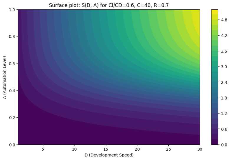
Fig. 1. Surface graph showing the relationship between delivery speed (S) and development speed (D) and automation level (A), under the conditions CI/CD = 0.6, C = 40, and R = 0.7

At a low level of automation (A < 0.3), an increase in D does not significantly accelerate delivery. The team continues to make changes, but the infrastructure struggles to keep up with the processing.

Only at medium and high automation levels (A ≥ 0.5) does the S curve exhibit a significant increase along the D axis. These findings support the multiplicative structure of the model. In such a model, the weakness of one factor limits the overall result.

This result is consistent with a well-known practical pattern. Increasing the speed of development is only effective when there is a sufficient level of automation in place.

Figure 2 shows graphs of S(A)'s dependence on complexity (C) at different levels. These graphs demonstrate the threshold and saturated nature of automation. In the model, this behavior is described by the logistic function E A (A).

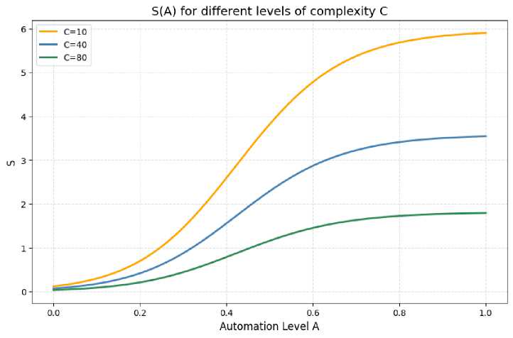
Fig. 2. Delivery speed (S) as a function of automation level (A) for different levels of system complexity (C)

In the early stages (A ≈ 0.1–0.4), a small increase in automation significantly increases delivery speed. Once average automation levels are reached (A ≈ 0.6–0.8), the increase in S plateaus. In this range, the system approaches its natural "ceiling".

This behavior is consistent with the empirical results of DORA and Accelerate. These studies found that the main effect of DevOps automation is evident in the early stages of implementation.

The S(CI/CD) graph shows a similar S-shaped curve. The transition from chaotic or partial integration (0-0.3) to basic CI/CD yields the most significant increase in S (see Fig. 3).

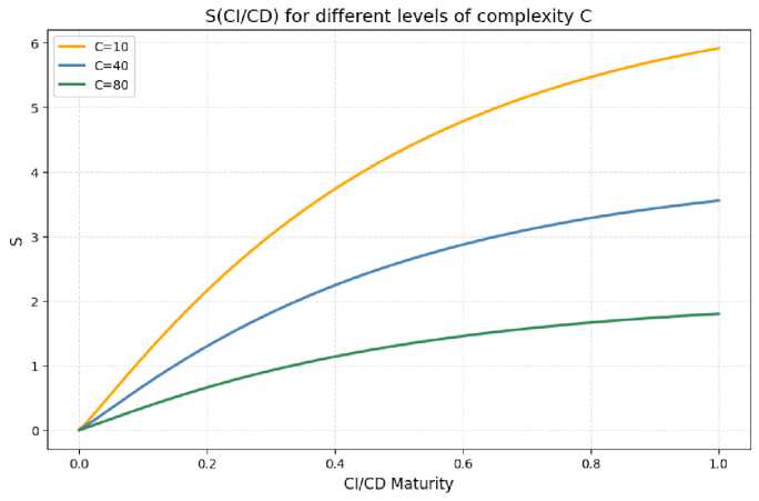
Fig. 3. Delivery Speed (S) Dependence on CI/CD Pipeline Maturity at Different Levels of Architectural Complexity (C)

Further increases in pipeline maturity (above 0.7) yield diminishing benefits, demonstrating the declining marginal utility of CI/CD. The model captures this concept mathematically through the exponential function in equation (8).

Thus, the model confirms an important practical pattern. The most effective CI/CD investment is creating a basic automated build, test, and deployment process. More complex optimization yields significantly less additional effect.

A separate graph of the S(C) dependency (Fig. 4) shows that complexity is the most critical negative factor in the model.

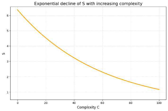
Fig. 4. Exponential Decrease in Delivery Speed with Increasing System Complexity

The delivery speed (S) decreases exponentially with increasing system complexity (C).

The exponential damping factor, e-λC, determines the rate at which delivery speed declines.

An increase in complexity from 20 to 40 units results in only a moderate decrease in S, whereas a transition from 60 to 80 units causes a sharp, nearly catastrophic decline.

This behavior is consistent with research on microservice architectures. The greater the number of services and interdependencies in a system, the more difficult it is for the team to maintain high delivery speed and stability.

A graphical representation of the model illustrates the intricate connections between the DevOps environment's essential parameters. These interrelationships highlight the model's nonlinear nature.

None of the factors operates in isolation. Automation, development speed, CI/CD maturity, resources, and architectural complexity are interconnected. Changing one parameter can significantly strengthen or weaken the influence of the others.

Automation and CI/CD do not work solely as positive factors. They also reinforce each other's effects. This synergistic effect is particularly noticeable when S increases with simultaneous increases in A and D.

Architectural complexity acts as a universal damper. When C increases, the positive effects of the other factors are significantly reduced. In some cases, this effect disappears almost completely.

The behavior of S is distinctly nonlinear. It contains areas of high sensitivity, threshold effects, and saturation regions. There are also areas of sharp performance decline. Linear models or individual metrics cannot explain this behavior. In the context of DevOps practices, this behavioral model is both logical and expected.

Accelerating development does not lead to faster delivery without proper automation and CI/CD maturity. This confirms the DevOps principle of not increasing the pace of change without first modernizing delivery processes.

Automation and CI/CD are the main drivers of throughput. However, even their capabilities have an upper limit. Beyond this limit, further improvements have minimal effect.

Architectural complexity, on the other hand, poses the most significant risk to delivery speed. Its growth reduces system throughput exponentially. This occurs regardless of the maturity level of other DevOps practices.

Resources produce a moderate stabilizing effect by mitigating bottlenecks and maintaining stable pipeline operation. The graphs do not display this effect, though the model's functional structure reflects it.

Thus, the simulation results confirm that the model is consistent with the basic principles of DevOps. The results also demonstrate the ability to quantitatively describe the complex interdependencies characteristic of modern engineering teams.

• 5.3.    Comparing the S Delivery Speed Model with DORA, CALMS, SPACE, and Accelerate

The S-model naturally fits into the current scientific and industrial discourse on evaluating the effectiveness of DevOps processes. At the same time, it differs from existing frameworks. The primary difference is that it offers a formal, quantitative representation of the interdependencies between key parameters.

The DORA, CALMS, SPACE, and Accelerate frameworks cover important aspects of DevOps maturity. However, these frameworks mainly present these aspects in the form of indicators, principles, or high-level recommendations. In contrast, the proposed S model enables the construction of functional dependencies. It also allows for scenario modeling.

In terms of DORA metrics, the proposed model accurately depicts the fundamental cause-and-effect relationships within the DevOps system. In the model, parameter D corresponds to deployment frequency. Parameters A and CI/CD determine the lead time for changes. This is because they control the level of automation and the maturity of the pipeline. Architectural complexity (C) and associated risk (Rsk) affect operational stability and the probability of failure. These parameters reflect the likelihood of failure and mean time to recovery (MTTR) metrics. The S-model formalizes the key components of DORA. It illustrates how technical and organizational factors influence the actual delivery speed. Thus, the S-model is consistent with DORA. It details its cause-and-effect structure. It also formalizes these relationships as mathematical dependencies.

In the context of the CALMS framework, the model represents its technical components. These components are Automation, Measurement, and Sharing. In the model, these components are presented as the quantitative variables A, CI/CD, and R.

The CALMS framework does not contain formal dependencies between complexity, automation, and delivery speed. Rather, the S model illustrates how nonlinear automation effects shape the throughput of the DevOps pipeline. It also illustrates the exponential impact of complexity on delivery speed.

The SPACE framework emphasizes team performance. This framework is consistent with the S-model. SPACE's factors of satisfaction, activity, performance, and efficiency correspond to the D, A, CI/CD, and R variables. However, SPACE lacks a mathematical apparatus for evaluating the integral result.

The S-model fills this gap. It allows you to quantitatively assess the effects of the interaction between technical and organizational parameters.

The Accelerate approach, on which DORA is based, emphasizes the importance of automation, continuous integration/continuous delivery (CI/CD), reducing cognitive load, and architectural modularity. In the S model, these factors are represented by parameters A, CI/CD, and C.

Accelerate's empirical findings demonstrate the diminishing marginal utility of automation. They also highlight the importance of architectural simplicity. The mathematical structure of the S-model confirms these findings. The logistic effect, EA(A), reflects the saturation of automation. The exponential damping, e-λC, reproduces the negative impact of complexity.

Table 3 compares the key characteristics of DORA, CALMS, SPACE, and Accelerate with the capabilities of S-model, which allows us to demonstrate its position among modern approaches. It also highlights the model's unique ability for quantitative analysis, forecasting, and educational applications.

Table 3. Comparison of Model S with Existing DevOps Frameworks

Aspect	DORA	CALMS	SPACE	Accelerate	Model S
Type	Empirical metrics	Cultural framework	Sociotechnical	Statistical	Mathematical
Quantitative dependencies	No	No	No	Correlations	Yes (functional)
Prediction	Limited	No	No	No	Yes
Saturation effects	Mentioned	No	No	Mentioned	Formalized
Architectural complexity	Indirect	No	No	Qualitative	Exponential damper
Calibration	No	No	No	No	Yes (MNK)
Educational application	Metrics	Principles	Framework	Cases	Simulations + laboratories

Therefore, the proposed S-model can be considered an extension of existing DevOps frameworks. It does not replace DORA, CALMS, SPACE, or Accelerate. Rather, it complements these frameworks with quantitative tools.

This apparatus allows for the analysis of various scenarios. It enables the calibration of parameters. It also allows for the evaluation of technical solution effectiveness. Additionally, it identifies nonlinear interdependencies that traditional metrics do not cover.

This approach opens up the possibility of integrating DevOps assessment with scientific-level system modeling.

• 5.4.    Implementing the S Delivery Speed Model in the Educational Process

The proposed S delivery speed mathematical model has significant practical value. It also has significant didactic value because it enables students of technical specialties to gain a deeper understanding of DevOps processes, their interdependencies, and the effect of technical solutions on organizational outcomes.

Unlike traditional approaches that focus on learning individual tools (CI/CD, Docker, Kubernetes, Prometheus, and Grafana), the S model offers a systematic view of DevOps. It considers DevOps as the interaction of parameters that shape the nonlinear speed, stability, and quality of delivery.

Using the model in the learning process has several important pedagogical effects. One such effect is demonstrating to students that technical solutions have a quantifiable impact on results and are not merely a set of practices or "best practices".

Thanks to formal dependencies, students can experiment with parameters such as development speed, automation, CI/CD maturity, resources, and complexity. They can also explore how the interaction of these parameters affects the final throughput. This promotes analytical thinking development. Students learn to interpret data and establish cause-and-effect relationships.

The S model can serve as the foundation for hands-on laboratory exercises in which students simulate the work of a DevOps team using synthetic or real data. Using Python and the Jupyter Notebook as standard tools for educational analytics and modeling enables students to calibrate the model independently, evaluate parameters, build graphs, and analyze nonlinearities and sensitivity zones. This format strengthens the research aspect of learning. Students act as both users of DevOps tools and researchers of processes.

Educators can embed the model in project courses where students develop DevOps pipelines and collect metrics. This enables them to compare their team's actual performance with the model's predictions. This approach fosters an essential skill: making data-driven decisions. This is a key principle of DevOps culture. By comparing the model with actual performance, students can identify bottlenecks and understand the impact of architectural complexity on their system. It also helps them explore the effects of automation and CI/CD, as well as evaluate delivery stability.

The S-model can be used to teach managerial and analytical competencies. Instructors can use scenario modeling to demonstrate the impact of various investments, such as those in automation, infrastructure, architectural optimization, and team expansion, on an organization's throughput. This approach is useful for students majoring in software engineering, computer science, information systems, and technology. It is also useful for future IT project managers.

The model promotes a culture of reflection and continuous improvement. It allows students to quantitatively see that not all technical improvements have the same effect. For instance, automation and CI/CD yield substantial gains in the initial stages. However, their effectiveness decreases as they approach maturity. Complexity has an exponentially negative effect. This reinforces the key DevOps principles of "shift left", "reduce cognitive load," and "optimize for flow".

Thus, integrating the S delivery speed model into the educational process enables us to transition from a fragmented study of tools to a system-oriented DevOps training approach. With this approach, students learn the technologies and the mechanisms by which they impact the productivity of engineering teams.

This approach aligns with current international trends in DevOps education. It contributes to developing the high-level competencies required for working in complex digital ecosystems.

As part of the "Information Systems Deployment" course for students majoring in "Information Systems and Technologies" at Lviv Polytechnic National University, the proposed S delivery speed model was tested. The purpose of the testing was to verify whether the S-model reproduces real processes occurring in student DevOps teams. A second objective of the testing was to evaluate the model's effectiveness in developing competencies in DevOps process analytics. This allowed us to assess students' understanding of the interaction between technical parameters and their impact on delivery speed.

During lab classes, students developed their own CI/CD pipelines using GitHub Actions and Jenkins. They deployed test applications in Docker and Kubernetes, performed automated testing, monitored systems, and collected metrics on delivery time, the number of releases, and service stability.

As a result, we compiled a set of empirical training data. This data characterized the work of eight student microteams over the course of four academic weeks, for a total of 32 observations. The data included the following indicators: D, the number of releases per week (range: 2-11); A, the proportion of automated steps in the pipeline (0.20.85). The CI/CD indicator, which measures pipeline quality and stability on a scale of 0.1 to 0.9, was recorded separately. The R indicator, which reflects the number of available runners and the amount of allocated resources (0.41.0), was also considered. The C parameter reflected the architectural complexity of the training project (10-35 conditional units). The S indicator described the actual delivery time in normalized form (1/lead time).

Table 4. shows a fragment of the training data averaged across teams.

Week	D	A	CI/CD	R	C	S (empirical)
1	3.8	0.28	0.21	0.55	33	0.36
2	5.9	0.47	0.38	0.63	28	0.82
3	8.2	0.58	0.55	0.71	22	1.41
4	9.7	0.72	0.71	0.84	18	2.05

After collecting the data, the students entered it into the S-model and compared it with the empirical S values, which showed a high level of agreement.

On average, there was a 14.3% deviation between the model values and the empirical indicators. This level of deviation is acceptable for small-scale educational projects with variability in student practices. The smallest deviation was observed in weeks with high automation (A > 0.5). This result is consistent with the model structure and real DevOps data. It is particularly important that the students can interpret the deviations. They identified several causes, including unstable tests, manual pipeline interventions, architectural changes, and temporary shortages of GitHub Actions resources. This confirmed that the S-model serves as a practical reflection tool for DevOps processes, not merely a theoretical demonstration.

The trial also demonstrated a significant pedagogical impact. Students began to perceive DevOps as an interconnected system rather than a set of separate tools. They understood that speed, stability, and quality depend on the interaction of various factors. The model enabled them to predict the consequences of technical decisions. Students saw that reducing the complexity of C by breaking down the monolith into modules and eliminating duplicate logic enhances the effect of automation and CI/CD. This helped them understand the importance of architectural decisions on the outcomes of the DevOps team.

6.    Conclusion

The article proposes a formalized, mathematical model of software delivery speed (S-model) that describes the interaction of key DevOps environment parameters: development speed (D), automation level (A), CI/CD pipeline maturity, resource provisioning (R), and architectural complexity (C).

Unlike qualitative or empirical approaches, such as DORA, CALMS, SPACE, and Accelerate, the S model provides a quantitative basis for analyzing DevOps processes. This allows one to predict how they will behave under different conditions. The model also enables the description of the nonlinear structure of DevOps processes. It considers threshold effects and the diminishing marginal utility of individual factors.

Analytical justifications demonstrated that the model's multiplicative nature accurately reflects the synergistic nature of DevOps. No parameter operates in isolation; the weakness of one factor can significantly reduce overall throughput. Introducing power elasticities makes it possible to assess S's sensitivity to changes in individual parameters. Using saturation functions and exponential damping allows us to model the behavior of automation and CI/CD at different maturity levels, as well as the adverse, accelerated effect of complexity.

Calibrating the model using pseudo-real data from the DevOps team confirmed its performance and demonstrated its ability to reproduce realistic dependencies. The estimated coefficients are interpretable. Automation and CI/CD have a strong, albeit saturating, effect, while development speed has a sublinear effect. Resources have a moderate stabilizing effect. Complexity is the most critical negative factor, exponentially reducing delivery speed. The high value of the coefficient of determination indicates the model's adequacy. This remains true even when using synthetic data.

Graphical analysis of the model confirmed the presence of sensitivity zones, threshold effects, and saturation areas. Traditional linear models do not reflect these characteristics. The S-model reveals significant patterns in DevOps practices. Increasing development speed without sufficient automation is ineffective. CI/CD provides the most significant benefit at initial levels of maturity. System complexity poses the greatest risk to delivery speed and can negate the positive impact of other factors.

Unlike DORA, CALMS, SPACE, and Accelerate, the S-model does not replace these frameworks. Instead, it acts as a quantitative supplement to them. The model clarifies the cause-and-effect relationships in traditional frameworks, presenting them as metrics or general principles. It also enables scenario modeling, forecasting, and the analytical assessment of the effects of technical decisions.

Testing the model in the "Information Systems Deployment" course at Lviv Polytechnic National University proved its high educational value.

Students could apply the model to their training data, perform calibration, interpret deviations, and identify cause-and-effect relationships in their DevOps projects. A comparison of the model's predictions with empirical values yielded a deviation of 14.3%. This is an excellent result for educational DevOps teams, confirming the model's practical applicability.

However, the S-model has certain limitations that determine the directions for further research. Calibration was performed using pseudo-real and small-scale training data. This requires verification in industrial DevOps teams with complete metrics. Additionally, the model does not consider socio-technical factors, such as team satisfaction, communication, and burnout. These factors can significantly impact productivity. Additionally, the model is static and does not describe the temporal dynamics of changes in DevOps processes. Future research could expand upon this aspect.

In summary, the proposed S-curve delivery speed model is a new quantitative analysis tool for DevOps processes. It combines mathematical formalization, calibratability, visual representation, and pedagogical value. The model can be used to study the effectiveness of DevOps practices and support technical decision-making. The model is also suitable for managing complexity, optimizing engineering processes, and preparing students to work in modern digital ecosystems.

The model lays the foundation for further research. First and foremost, this concerns extending it to operational stability, product quality, and risk management. With access to complete DevOps metrics, the model can be used in real production environments.