Mathematical modeling of the thermal condition of pressurized aircraft compartments

A mathematical model of the thermal state of sealed compartments of a supersonic passenger aircraft describes the process of heat transfer through aircraft structures, heat generation or heat absorption by on-board equipment, air conditioning systems [1–4].

The parametric identification of the mathematical model of the thermal state of sealed compartments relates to the solution of ill-posed problems in the mechanics of viscoelastic media [5] using numerical analysis methods for mathematical models [6].

The use of cellular fuselage structures is a promising trend in the field of aviation technology [1; 7; 8].

The criteria for optimizing the thermophysical characteristics of the sealed compartment are determined in accordance with the AP 25 airworthiness standards [9].

Mathematical model of the thermal condition of aircraft compartments

Solving the problem of optimizing the thickness values of cellular structures in sealed compartments requires determining the thermal state of the compartments. The mathematical model of hermetically insulated on-board compartments with an air conditioning system is represented by the equations of heat exchange between the skin and the air in the insulated compartments, taking into account the heat transfer of on-board equipment, as well as heat transfer from the air conditioning system to the compartments.

The heat transfer equations of a multilayer heterogeneous honeycomb cladding structure for boundary conditions of the third kind are presented in the form of heat conduction equations describing the process of heat transfer in a heterogeneous structure. The thermal conductivity of a heterogeneous structure will be equal to the thermal conductivity of a honeycomb structure calculated for boundary conditions of the first kind of a parabolic boundary value problem with discontinuous coefficients.

The mentioned equations have the following form [10, 11]:

C cv ( x) T cv,t = (4 v ( x ) T cv, x ) x , 0 <  x <  l hon , 0 <  t ^ t k ;                        (1)

^λcv ⁽ x ^{) F} cv,in ^T cv, x

α cv,out ( t ) F cv,in ( T cv,out ( t , x ) - T e (t )) + Q cv,out ,

x = 0;

^λcv⁽ x ^{) F} cv,in ^T cv, x

^acv,in ⁽ t ) F cv,in ⁽ T arpr ⁽ t )   T cv,in ⁽ t ^{, x} )) ⁺ Q cv,in^,

x = l ;

T cv (0, x ) = T o ( x ), 0 <  x <  l hon ,                                    (4)

where C _cv ( x ) =

x g hon ;

x g air ,

λhon , λair,

x g hon ;

x g air ,

that is, the coefficients C _cv , λ_cv they depend on which layer the heat transfer is considered in.

Equations (1) to (4) use the following notations: T _cv ( t , x ) – temperature of the honeycomb structure; T _cv,t – the first derivative T _cv on t ; t – time; T _cv,out – the first derivative T _cv on x ;

Tcv,x,x – the second derivative Tcv on x ; Tcv,out, Tcv,in – the temperature of the outer surface of the honeycomb structure and the inner, respectively; lhon – the thickness of the honeycomb structure; Ccv(x) – volumetric heat capacity of the honeycomb cladding structure, determined by the heat capacity of duralumin Сhon and the heat capacity of the air Сair ; λcv(l) – thermal conductivity of the honeycomb structure, determined by the thermal conductivity of duralumin λhon and the thermal conductivity of the air λair ; αcv,out – heat transfer coefficient of the outer surface of the honeycomb structure; αcv,in – heat transfer coefficient of the inner surface of the honeycomb structure; Fcv,in – the area of the honeycomb structure during external and internal heat exchange; Qcv,out – thermal energy from external sources; Qcv,in – thermal energy from internal sources; Te – recovery temperature; Tair,pr – the temperature of the air environment in the sealed compartment or in part of the compartment; Tj – temperature of the j-th compartment element; l – the thickness of the honeycomb structure.

Forced convection outside the sealed compartment and boundary conditions of the third kind . Heat transfer coefficient α _cv,out the outer surface of the skin will be calculated using the formula [10]

a cv,out = 3,26(Re Out ) ^{- 0,}5 (Pr *ut ) ^{- 0,66}6 P * c * * air,out

for a laminar boundary layer under the Reynolds criterion Re*out < 1·106 and according to the formula [10]

a cv,out = 0,181(lg Re Out ) ^{- 2,584} (P^ t ) ^{- 2}/³ P * c * J ..                                   (6)

for a turbulent boundary layer under the Reynolds criterion 1^10 6 <  Re_out <  1^10 9 .

In the equations (5), (6) the following notation is used in the equations: Re*out , Pro*ut – the

Reynolds and Prandtl criteria for air temperature, respectively T ^* ; ρ _V ^* – the density of the air outside at temperature T ^* ; c _p ^* – specific heat capacity of air at temperature T ^* ; V _air,out — airspeed of flight.

Air temperature T ^* it is determined by the formula

*

T = Tair,out + 0,72(Te - Tair,out) , where Tair,out — the temperature of the air outside the thermal boundary layer.

Criteria Re*out calculated using the formula

***

Reout = Vair,out pV A^out/^air ’ where Lcv,out – typical size for the outer surface of the skin; μ*air – dynamic air viscosity.

Characteristic size L _cv,out it is assumed to be equal to the distance from the nose point of the fuselage to the middle of the calculated compartment or part of it.

Dynamic viscosity μ*air it is defined by the expression

μ*air = 0,1222229∙10–6 + 0,682674∙10–8 T* – 0,313155∙10–11 (T*)2.(9)

Criteria Pro*ut calculated using the formula

Prout = c Xir/Cr , where λ*air – thermal conductivity of air.

Thermal conductivity λ*air it is defined by the expression

λ*air = 0,141483∙10–2 + 0,896161∙10–4 T* – 0,204759∙10–7 (T*)2 .(11)

Air density ρ _V ^* overboard is calculated by the expression

P V = 3,4826 -10 ³ p air,out / T,                                       (12)

where p _air,out – air pressure overboard.

Recovery temperature T _e in equation (2), it is determined by the expression

T e = T air,out (1 + M ² r ( k ~ 1)/2),                                       (13)

where r - temperature recovery coefficient for laminar boundary layer r = Pr_out , for turbulent - r = 3 Pr_ou t ; M — the Mach number at the outer boundary of the boundary layer; k = c p / c_v - the ratio of the specific heat of a gas at constant pressure and volume.

Forced convection in a sealed compartment and boundary conditions of the third kind . Heat transfer coefficient α _cv,in The inner surface of the honeycomb structure can be calculated using the formula [11]

a cv,in = 0,66 ^ Re in ⁵ Pr?' / 4v,_m                           (14)

for a laminar boundary layer under the Reynolds criterion Re_in < 4∙10⁴ and according to the formula [11]:

a cv,in = 0,037 ^ air Re '? Pr in’43 / L cv,in                                 (15)

under the Reynolds criterion Re in >  440 8 .

Thermal conductivity λ_air and dynamic viscosity μ_in in formulas (14), (15) in the criteria Re _, Pr they are defined according to the expressions (11), (9) for the air temperature in the compartment T _air .

The product of J_W of the density ρ _air and velocity W _air of the air in the compartment or the mass velocity J_W in the criterion

Re in = P air W air L in / P air                                            ⁽¹⁶⁾

it is accepted from the results of the experiment.

The characteristic size L _cv,in is assumed by analogy with L _cv,out the equal distance from the beginning of the compartment to the middle of the calculated part of the compartment.

The process of heat transfer through a sealed thermally insulated partition between a sealed thermally insulated and an unpressurized non-insulated compartment is represented in the form of onedimensional equations of thermal conductivity

Cbi (x) Tbi,t = (X bl (x) Tbi,x)x, 0 < x < l, 0 < t < tk;(17)

X bl(x) Fbi, uprTbl, x a bl, upr (t) Fbl, upr (Tbi(t) — Tair, upr (t, x))’ x 0;(18)

X bl (x) Fbl, prTbl, x =a bl, pr (t) Fbl, pr ( Tair, pr (t) - Tbl (t, x)), x = l;(19)

Tbl (0, x) = T0(x),     0 < x < l,(20)

где C bl ( x ) =

C compo , x e compo ;

C air , x e air ,

X ы ( x ) =

X compo , x e compo ;

X_a ir , x e air .

Equations (17) – (20) use the following notations: T_bl ( x , t ) – temperature of the honeycomb partition; T_{bl ,t} is the first derivative T_bl on t ; T_{bl , x} is the first derivative T_bl on x ; T_{bl , x , x} is the second derivative T_b l on x ; C_b l ( x ) - bulk heat capacity of the partition; X bl ( l )- thermal conductivity of the partition; a _b l , upr , a bl , pr - heat transfer coefficients of the partition surface from the side of the unsealed and sealed compartments, respectively; F_{bl , upr} , F_{bl , pr} – the area of the partition participating in convective heat exchange from the side of the unpressurized and pressurized compartments, respectively; T _{air, upr} – the air temperature in the unpressurized compartment or in a part of the compartment.

The process of heat transfer of on-board equipment is represented as an ordinary differential equation describing convective-radiation heat exchange with surrounding structures

^Tm ,t ^a air, m ⁽ t ) F air, m / C m ^{( T} air, pr ⁽ t ) ^Tm ) ⁺

⁺ E g j , m / C m ^Tj ⁽ t ) / ^Tms ^{— c} 0 ^e m ^Fm / C m T mn ^{+ Q}m / C m ,

m where Tm is the temperature of the m-th airborne equipment; Tm,t is the first derivative Tm on t; Tms is the reference temperature; aair m is the heat transfer coefficient of the m-th on-board equipment; Fair,m is the area of m- th on-board equipment during convective heat exchange; Cm is the heat capacity of the i - th on-board equipment; c0 is the Stefan-Boltzmann constant; gj,m is the coefficient of radiative heat exchange of the system «j-th element of the compartment – m-th block of on-board equipment »; εm is the emissivity coefficient of the m-th block; Qm is the energy of heat release or heat absorption by the m-th on-board equipment, from the air conditioning system and converted from electrical energy.

We will represent the process of heat transfer of the compartment structures in the form of an ordinary differential equation describing convective-radiative heat exchange

Tr = = a„:r r (t)Fa:r r / Cr (Tajr (Г)t) — Tr) + r,t air,r air,r r air, pr r

+ E gj,r / CrTj (t) / ^s — c0 £rFr1 CrT4 + Qr 1 Cr, r where Tr is the temperature of the r -th structure; Tr t is the first derivative Tr on t; a air r - heat transfer coefficient of the r-th structure; F – area of the r - th structure in convective heat transfer; air,r

C_r – is the heat capacity of the r -th structure; Q_r – heat release energy of the r -th structure; g_{j , r} is the coefficient of radiation heat transfer of the system « j -th element of the compartment – r -th structure; e _r is the coefficient of blackness of radiation of the r -th structure.

The heat transfer of the air in a thermally insulated pressurized compartment is represented as an ordinary differential equation describing the convective heat exchange between the inner surface of the thermal insulation of the skin, on-board equipment, structures and the air in the compartment, as well as the transfer of heat from the air conditioning system to the compartment:

T air, pr ,t ^a cv,in⁽ t ) F v,in, pr / ^C air⁽ T cv,in, pr ^{( l} cv, pr ’ t ) T ir, pr ) ⁺

^{+ a} bl , pr ⁽ t ) F bl , pr / C air ^(Tbl , pr ^{( l}bl , pr , t ) ^— T air, pr ) ⁺

■E >  •-. r ( t ) F air, r / C air ( T ( t ) — T air, pr ) + Q r / C air ) + r

E^ , p ( t ) F air, p / C air ( T p ( t ) — T air, pr ) + Q p / C air ) ^p

⁺ Е ^{( а} о^, m ⁽ t ) F air, m / C air ^{( T}m ⁽ t )   T ir, pr ) ^{+ Q}m / C air ) ⁺

m

Baarr,j(t)Fair,j / Cair(T(t) — Tair,pr) + CpGstm / O^stm — Tair,pr), j where Tair, pr,t is the first derivative Tair, pr on t; Gstm is the expense of air following from a central air; Tstm is the temperature of air following from a central air; Tcv,in, pr – temperature of an internal surface of a covering in a pressurized compartment.

The thermal capacity of air C _air is defined on expression

С air    ^c p ^{( p} air G stm ^A t ^{+ p} air ^ air ),

where pair - air density in a compartment; cp - heat capacity of air at temperature; A t - an interval of digitization of time at the decision of system of the differential equations; Vair – air volume in a compartment.

The heat capacity of air C _air is determined by the expression (24).

Surface heat transfer coefficients α_cv,out , α_cv,in , α _{bl , upr} , α _{bl , pr} , α_{air, m} , α_{air, r} in equations (2), (3), (18), (19), (21) – (23) we will calculate using the methods described in [10-13].

The coefficient of radiative heat transfer in equations (21), (22) is determined by the Monte Carlo method [14].

Algorithm for solving the direct problem of the thermal state of the honeycomb structure of the sheathing

To solve the direct problem of the thermal state of the honeycomb fuselage structure, let us consider the mathematical model of heat transfer in the heterogeneous structure (1) – (4), (17) – (20) as a parabolic boundary value problem with discontinuous coefficients. A description and physical properties of heterogeneous structures can be found in [15].

Heat transfer in a heterogeneous structure is described by the following parabolic equation

°— - X '    a j ( t , x ) = 0, ( t , x ) ^€ Qt ,                           (25)

dt x dx,

• i , j = 1 i \                J 7

where is Q - = (0, t k ) x G ; - ( t, x ) - the temperature of the structure; a ij - coefficients that are

Lipschitz continuous in functions in subdomains G(k), k = 1,...,M . In the case of a honeycomb panel aij the coefficients are the coefficients of temperature conductivity

4v( x )

a ij ( t , x ) = Ccv⁽x)

i = J ,

0, i ^ J .

The coefficients a ij are separated by surfaces in the areas Г , that in each cell are the interfaces between the air and the frame made of carbon fiber

^ X ^ 2 <  X a ij ( t , x )^ j < n X ^ • i i , j                                   i

It is also required that the function you are looking for satisfies the condition:

^- t = o = Ф^{( x} )

and boundary condition on d G :

X a ij n i I i , J

5 -

— + n ⁽ t , x ) ^- + Y ⁽ t , ^x ) d x j

= 0 .

x eS G

In [16] the existence of generalized solutions to boundary value problems (25), (27), (25) and (29) is proved. Moreover, these solutions can be approximated by solutions of the corresponding boundary value problems with coefficients that are approximations of the initial discontinuity coefficients. For example, you can get an approximate solution to the original problem by solving a problem with smoothed coefficients. In this paper, it is proposed to statistically estimate the solution of the problem with smoothed coefficients using a method based on the numerical solution of stochastic differential equations and, thus, to obtain estimates of the approximate solution of the initial boundary value problem with discontinuous coefficients.

To smooth out the coefficients, it is proposed to use integrative averaging [16; 17] f ^{(p) ( x} ) = p ^-3 j ю _р (| ^x - y I) f ⁽ y ) dy                                 ⁽³⁰⁾

Ix - y I

p and j Ир(| ^ |)d^ = 1 . In (19) onwards p the averaging radius, and the symbol |a| denotes the Euclidean I ^p norm of the vector a .

Estimation of the solution of the boundary value problem for a parabolic equation with discontinuous coefficients based on the numerical solution of stochastic differential equations

The solution of a parabolic equation can be represented as a mathematical expectation of the functional for solving stochastic differential equations [17]. This fact can be used to obtain statistical estimates of the solutions of parabolic equations using the numerical solution of stochastic differential equations. An approximate solution to the problem in this way can be obtained at one or more points within the region, which is often sufficient for practical application. At the same time, there is no need to build a grid from spatial variables and solve large systems of linear algebraic adjustments. The method of statistical modeling is easily parallelized with high efficiency. Therefore, supercomputer technology can be used to solve the problem. We use this method [18] to estimate the solution of a parabolic equation with smoothed coefficients obtained on the basis of integral averaging (30).

The approximate solution of equation (25) will be found as the solution of the following equation

S T      5    (p) 5 T

- 0,

, - E У a ij й

д t дх,- дXj

1, J-1    1 \ J J where aj are the smoothed coefficients of equation (25) in the neighborhood Г . Accordingly, the boundary condition corresponding to the smoothed coefficients has the form

(

E a j n i    ⁺ П ⁽ t , ^x ) T + Y ⁽ t , ^x )

I i , J j     ^{д X}J                        J

- 0.

x eS G

For a point ( t , x ) e Q t we define a stochastic process X • , that starts motion from a point x at a point in time t and which is the solution of the following vector stochastic differential equation [19; 20]

X v - x + j b ( X r , r ) dr + j о ( X_r , r ) dW r + j n A ( X_r , r ) d | k_r |,                 (33)

T-t                    T-t                        T-t where W• is the Wiener process [16]; nA is the normalized vector of internal conormality, i.e.

v nA - An/ | An |; | kv |- j 1sg (Xr)d | kr | - a non-negative random process that grows only when the t process X• reaches the boundary; о - (3 x 3) is a matrix such that, 2oTо - A(p),

A^(p) - ( a ^) ; b -X a

( i - 1

S x i

у S a? ’ ^{E S} x i

у Мз).

’ ^E S x,

I - 1       i J

In addition, let's introduce notations: E _{t, x} mathematical expectation relative to a probabilistic measure P _{t, x} , corresponding to a random process originating from a point x at a moment in time t ;

1 _S is a function of the set S .

In addition, let's introduce notations: mathematical expectation relative to a probabilistic measure corresponding to a random process originating from a point at a moment in time; is a function of the set.

Thus, we can obtain estimates of the solution of problem (31), (32), (28) by numerical simulation of the trajectory of the process X _• . To do this, we use a modified Euler method, according to which approximate trajectories X _• are calculated according to the formula [21]

^xi + 1 ^{- x}i ^{+ hb ( x}i , t i ) ^{+ 00 o( x}i , t i ^)Z i ⁺ ( ^A i + 1 K ) n A , t i + 1 ^- ti ^{+ h} , ⁽³⁵⁾

Ai+iK -[d (Xi + hb(xi,ti) + 00o(Xi,ti)Zi)] , (36) where nA is the unit vector of the internal conormal at xi, if xi it is on SG; [ a ] - max {0, - a}; d (x) is a nonpositive real function satisfying for any point x ^ G the following equation x - p(x) + d(x)nA(p(x)) (37)

Equation (37) uses the following notations: p( x ) - projection of a point x £ G on G * in the direction of the conormal; n^A (ρ( x )) is the single vector of the internal conormal in ρ( x ) . Note that d ( x ) = 0 , if x e G .

To obtain an approximate solution (estimate) of the problem (31), (32), (28), it is also necessary to calculate the following functions defined on the time grid

1, i = 0, yi =

( i-1                                  У exP E П(tk, xk )15G (xk )Дk+1K , i ^ 1,

\ k = 0

0, i = 0, zi =

i -1

E ( Y ⁽ t k , x k )1 s G ⁽ x k ^)д k + 1 K ) y k , i ^ 1-

I k = 0

The assessment of the solution of the problem (20), (21), (15) is determined by the formula

^{T (} t , x ) = E t k -t, x [ ф ( x N ) y N + z N ] ,                                 ⁽³⁹⁾

Algorithm for solving the direct problem of the thermal state of the internal elements of the compartments

The obtained equations (21)–(23), which describe the heat exchange of the internal elements of the compartments, constitute a rigid system of ordinary differential equations. This system of equations can be written in general as follows:

Y t = F ( Y ( t , 0 )), t e (0, 1 1 ); Y t = Y ₀ , F , Y e R S ; 0 e R^r ,

where Y = [ T cv , T bi , T m , T_r ,... ] ^T - a vector of parameters of a thermal condition of a compartment; Y _t — a vector of first derivatives Y on t ; © = [ Up и 2 ,... , и 5 ] ^T - a vector of factors of model; T – the top index designating operation of transposing.

For the decision of the equation (40) it is offered to use the following numerical scheme of Rosenbrock type of the second order of approximation for on-line systems [22]

^Y n + 1 = ^Y n ^{+ aK}1 + ^{(1 -} a ) ^K 2^;

K 1 = h ( I - ah ^ _Y ( Y n , t n , © )) ^{- 1} Ф ( Y n , t n + ah , © );

K2 = h(I - ah Фу (Yn,tn,©))-1 Ф(Yn,tn + aK 1,tn + 2ah,©); a = 1 —1/^2, where Yn, Yn+1 - the decision of the system received on n and (n + 1) iterations, accordingly; Ф - the Algorithm for parametric identification of the mathematical model of the thermal state of the honeycomb structure right part of system; ΨY – Yakobi matrix; I – an individual matrix; h – an integration step.

Algorithm for parametric identification of the mathematical model of the thermal state of the honeycomb structure

The inverse problem solution, that is, the estimation of the 0 model (1) - (4), (17) - (20), reduces to minimization of the discrepancy squares weighted sum between the values Y obtained during the calculations by the model equations Y (t, Θ) , obtained during the calculations by the model equations:

G means closure G

N

Ф ( @ ) = £ ( Y k - Y k (t k , © )) T ( Y k - Y k (t k , © )),                        (44)

k = 1

where t_k – are time points at k = 1,...,N.

We will determine the minimum of the function Φ ( Θ ) with the help of the iterative minimization algorithm that uses the derivatives of function Φ ( Θ ) . For this purpose, it is proposed to use the variant of a stochastic quasigradient algorithm with a variable metric [23], in which the approximations to the minimum point are constructed by the rule

Θ ^{k + 1} = Θ ^k - ρ _k Η ^k ∇ ^k Φ , k = 0,1,K,                            (45)

where Hk - is a random square size matrix of order l x l; VkФ - the gradient of the objective function at the point Θk; ρk – the step parameter.

The sequence of matrices Η ^k is calculated according to the scheme: Η ⁰ = I , Η ^{k + 1} + ( I - μ _k ∇ ^{k + 1} Φ ⋅ ( Δ ^{k + 1} Θ ) ^T ) Η ^k , _Δ k + 1 _{Θ = Θ} k + 1 _{- Θ} k _.

the constant,

The parameter μk is chosen from the equation μk = μ/( ∇k+1Φ ⋅ Δk+1Θ , where μk such that 0 < μk <1.

At each step of the algorithm, the step parameter ρ _k . is automatically adjusted. If

Ф(0k+1) > Ф(0k), то pk+1 = pk /y, где Y > 1 is a fixed parameter. If Ф(0k+1) < Ф(0k), then the following sequence of actions is performed: pk i = pk Y, 0k+1,i =0k - pk i Hk Vk Ф, and calculation Φ(Θk+1,i), i = 0,1,K.

These actions are performed as long as the value of the function Φ(Θ) decreases and the following conditions are fulfilled: ρmin ≤ ρk,i ≤ ρmax (ρmin,ρmax – minimum, maximum step length, respectively) and i < imax (imax – is the specified maximum number of iterations for increasing the step). The values Θk+1, ρk+1 are set equal to the values Θk+1,i, ρk,i , respectively, which are equal to the minimum value of obtained in such a way values of Φ(Θ) .

Algorithm of parametric identification of the mathematical model of the thermal state of the internal elements of the compartments

Algorithm of parametric identification of the mathematical model of the thermal state of the internal elements of the compartments

Parametric identification of the thermal state model of other elements (21) – (23). is proposed to perform using the composition of the steepest descent method.

As it has been noted in [23], for minimisation of function (44) it is expedient to use method of fastest descent [24], Brojdena – Fletchera – Goldfarba – Shenno’s quasi-Newton method [25] in a combination to Newton's method [26], which is realised according to the formula:

Θ j + 1 = Θ j + a j ⋅ S ( Θ j ),                                      (47)

where a_j – the factor characterising length of a step on j iterations; S – the parameter specifying a direction of search of a vector Θ ₀ of the valid values of factors Θ .

Next direction S of search of j vector Θ in this algorithm is defined from system of the equations: ∇ ² Φ ( Θ _j ) ⋅ S ( Θ _j ) =- ∇Φ ( Θ _j ),                               (48)

where ∇ ² Φ ( Θ _j ) - ( r × r ) – the Gess matrix representing a square matrix of the second private derivatives of function Φ on a vector Θ ; ∇Φ ( Θ _j ) – градиент функции Φ в текущей точке Θ _j .

Initial matrix ∇ ² Φ ( Θ _k ) in the equation (48) has been accepted by the individual.

For the decision of system of the equations (48) matrix ∇ ² Φ ( Θ _j ) is represented in the factorized to the form:

∇ ² Φ ( Θ _j ) = L ( Θ _j ) D ( Θ _j ) L ^T ( Θ _j ),                              (49)

where L ( Θ j ) – low triangle matrix with an individual diagonal; D ( Θ j ) – a diagonal matrix.

Matrixes L ( Θ _j ), D ( Θ _j ) receive decomposition Holessky matrixes ∇ ² Φ ( Θ _j ) on the algorithm described in [25].

To minimize the function (44) by the quasi-Newtonian method of Broyden-Fletcher-Goldfarb-Shenno, the next direction of search Θ _j is determined from the system of equations (48).

The estimation of the Hesse matrix of the second partial derivatives in this algorithm is carried out according to the Broyden-Fletcher-Goldfarb-Shenno formula [25].

In the process of minimization using a quasi-Newtonian al-gorhythm, gradient calculations of the function are required at each iteration ∇ ² Φ ( Θ _j ) .

The components of the gradient of function (48) are computed by the formula

N

∂ Φ / ∂ ϑ 1 = 2 ∑ ( Y k - Y k ( t k , Θ )) ^T ∂ Y k ( t k , Θ )/ ∂ ϑ 1 ,                      (50)

k = 1

where H _{1, k} = ∂ Y ^ˆ _k ( t_k , Θ ) / ∂ ϑ ₁ are derivatives of the solution of equations (21) – (23) by ϑ ₁ , which are called sensitivity functions [25].

Application of the algorithm (47) – (50) to the system (21) – (23) and sensitivity functions

Y _{t , Θ} = f _Y Y _Θ + f _Θ ,

Y Θ ( Θ ) = 0,                                        (51)

requires the calculation of a system of size equations at each step S × ( r + 1) .

In system (51) f _Y is the matrix of the first partial derivatives f in Y size S × S . f _Θ is a matrix of the first partial derivatives f by Θ size S × r . The matrix of the system (51) contains blocks on the main diagonal I - ah f _Y , and in the first columns S there are elements that include derivatives f _{Y , Y} and f _{Y , Θ} ; f _{Y , Y} is a matrix of the first partial derivatives of Y the elements of f _Y the size matrix S × S × S ; f _{Y , Θ} is the matrix of the first partial derivatives of Θ the elements of the matrix f _Y dimensions S × S × r .

The described algorithm was studied by numerical modeling for a number of specified (reference) values of the vector of the flight mode parameters U = [ρ _V , V _air,out, T _e] ^T (where ρ _V is the density of the air environment overboard; V _air,out is the airspeed of flight; T _e is the recovery temperature) and the desired coefficients Θ ₀ , which were correlated with the calculated values of the measurement vector by (21) – (23) and noisy values Y . The stability, speed and accuracy of the algorithm's convergence were studied depending on the form and accuracy of setting the initial conditions and other factors. At the same time, the quality criteria were the values of the residual function Φ ( Θ ) of the last iteration and the values ( Θ ^ˆ _j - Θ ₀) / Θ ₀ , that determine the uncertainties of the coefficient estimates Θ ^ˆ relative to their actual values Θ ₀ .

Based on the results of the simulation, we concluded that the proposed algorithm is satisfactory. The final results are insignificantly dependent on the uncertainties of setting the initial values of Θ _int .

The adequacy of the constructed model to real processes was checked using the method of residue analysis [26] for the case of additive random uncorrelated uncertainties distributed according to the normal law, and for the case of arbitrary statistical properties of the uncertainty vector.

The results of the model adequacy check are given in Fig. 1.

In determining the uncertainties of the obtained estimates, we introduced [26] some conditional joint confidence intervals ΔΘ of each of the desired coefficients in the form of projections of the joint trust domain on the corresponding coordinate axes of space Θ , which is equivalent to replacing the elliptic region with a parallelepiped described around it.

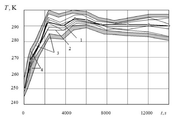
Рис. 1. Сопоставление рассчитанных и измеренных значений температуры Tair, pr в отсеке летательного аппарата:

• 1    – реализация средних арифметических рассчитанных в нескольких точках значений температуры; 2 – рассчитанные значения температуры; 3 – границы измеренных в нескольких точках значений температуры; 4 – доверительные интервалы неопределённостей измерений

Fig. 1. Comparison of calculated and measured temperature values T _{air, pr} in the aircraft compartment: 1 – implementation of arithmetic averages calculated at several points of temperature values;

• 2    – calculated temperature values; 3 – boundaries of temperature values measured at several points;

4 – confidence intervals of measurement uncertainties

Estimation of the coefficients of the mathematical model of the thermal state of the nose instrument purged compartment

A supersonic aircraft was accepted as the object of research (Fig. 2).

The parameters of the flight mode and the air environment overboard of the aircraft application model are shown in Fig. 3.

The takeoff path runs from the starting point to the initial climb of 10 m above the takeoff surface.

Then, at an altitude of 450 m, the transition from takeoff to the route flight configuration takes place.

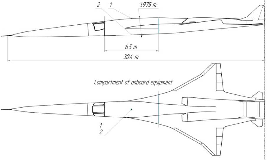
Рис. 2. Размещение бортового оборудования на сверхзвуковом летательного аппарата

• Fig. 2.    Compartment of onboard equipment on a supersonic aircraft

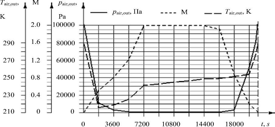
Рис. 3 . Параметры режима полёта и воздушной среды за бортом модели применения летательного аппарата:

pair,out, Па;        М;          Tair,out, К; pair,out – давление воздуха за бортом за пределами теплового пограничного слоя; M – число Маха на внешней границе пограничного слоя;

• Fig. 3.    Parameters of the flight mode and air environment overboard the aircraft application model:

p air,out — air pressure outside the thermal boundary layer, M – is the Mach number at the outer boundary of the boundary layer; T air,out is the air temperature overboard outside the thermal boundary layer

The characteristics of the on-board equipment units located in the compartment are presented in Table 1.

Table 1

The characteristics of the on-board equipment units located in the compartment

Part number of the compartme nt	On-board equipment unit number	Area heattransmittingsurface of the block F air, i , m 2	Block weight m, kg	Heat release energy of the block Qi , W
I	1	0.081	1.0	0
	2	0.330	3.5	41
	3	0.230	18.0	1200
	4	0.124	2.5	180
II	5	0.488	10.0	100
	6	0.125	8.6	378
	7	0.180	8.5	27
	8	0.325	8.5	66
	9	0.450	10.0	38
	10	0.249	6.0	60
III	11	1.005	35.0	463
IV	12	0.105	3.0	50
	13	0.081	1.0	0
	14	0.054	8.0	0
	15	0.054	8.0	0
	16	0.273	4.5	146
	17	0.762	25.0	400
V	18	1.151	36.0	430
VI	19	0.984	40.0	285
VII	20	0.530	14.0	15
	21	0.390	12.0	600
VIII	22	0.118	3.3	15

For the cold climate the initial air temperature should correspond to 283.15 К. For the extremely warm and dry climate, the initial air temperature should be 315.15 К. The temperature of air at the exit from the air conditioning system in flight should not be less than 276.15 K and more than 335.15 К.

Air flow rate of compartment air conditioning system G_stm it is proposed to represent a linear regression of the form

G stm ( t ) = ^ G ,0 + ^ G ,1 P v ( t )M 2 ( t ), (52) were fy Go , & Gi — model coefficients to be evaluated.

The model coefficients vector (1) – (4), (17) – (20), (21) – (23) when optimizing the thermophysical parameters of air conditioning, as well as the heat insulation thickness of the compartments has the following form:

Estimations of factors of model for cold and extreme warm dry climate types are accordingly equal to

Θ = [0.06 275.7 0.002 0.001] ^T .

Vector P _D uncertainties estimates Θ is equal to at confidential probability β = 0.99 accordingly

P _D = [0.008 3.7 0.0008 0.00007] ^T .

Conclusions

A method is proposed for characterization of honeycomb structures and the air conditioning system of the aircraft onboard equipment on the basis of the developed mathematical model aircraft pressurized compartment thermal state.

Determination of the honeycomb structure thermal state is carried out by a combined method in which the calculation of the diffusion process trajectories in cells filled with air is carried out by the random walk by moving spheres method, and along the framing, bounding plates and in their close neighborhood by the Euler method.

In the parametric identification of the onboard equipment housing honeycomb structure thermal state mathematical model, a stochastic quasigradient algorithm with a variable metric is used.

The proposed method makes it possible to optimize the thermophysical parameters of the onboard equipment housing and the thermocontrol system during the onboard equipment design.

The adequacy of the model was checked by analyzing the balances.

The studies were carried out in accordance with the Airworthiness Standards of the Aviation Rules AP 25.