Matrix arithmetic based on fibonacci matrices

Theory of number systems is one of the most ancient mathematical theories. Historically number systems preceded to origin of number theory and were the first mathematical results influenced essentially on development of number theory and on forming of its basic notions. The discovery of positional principle of number representation considers as one of the greatest mathematical discoveries of the ancient mathematics. The history of the positional number systems began in the Babylonian mathematics. As it is emphasized in [1], "the first of the familiar number systems based on the positional principle was the sexagesimal number system of the ancient Babylonians emerged about 2000 BC".

Let us consider the representation of real number A in the positional number system:

A =∑ _i a_iRⁱ                                 (1)

where a_i is the numeral of the i- th digit ( i = 0, ± 1, ± 2, ± 3, …) of number system (2); R is a base or a radix of number system (2); Rⁱ is the "weight" of i- th digit.

Two basic properties are common for all positional number systems:

• (1)    each digit takes the values from the finite set M of the permissible values;

• (2)    the "weight" Rⁱ of each digit is the function of its position and of some constant called the base of the number system.

The history of arithmetic [1] shows that the properly positional principle did not change starting since the Babylonian sexagecimal number system. A progress of the positional number systems was connected with a change of their bases and the set M of the numerals used for number representation.

Historically there appeared first the positional number systems with the natural bases (2, 3, 10, 12, 20, 60, etc.). The first step for extension of the functional possibilities of the positional number systems was made by the American scientist Claud Shannon who introduced the number systems with the negative bases [2].

In 1957 the American mathematician G. Bergman introduced the number system with an irrational base [3]. A peculiarity of Bergman's number system consisted of the fact that Bergman used the number τ =

1 + V5

called the "golden section" or "golden ratio" as the base of his number system.

The number system with irrational bases based on the generalized "golden ratios" were introduced by the author of the present article in the 80th [4].

Let us note one peculiarity of the positional representation of (1) and its generalizations given in [3] and [4]. The expression of (1) gives only certain class of real numbers, which could be represented in the form of (1). It is clear that many irrational numbers, for instance the number of π , Euler's number of e cannot be represented in the form of (1). It means that the expression

Q =

1 1)

1 о ^J

Note that the determinant of the Q- matrix equals to -1.

In the paper [13] devoted to the memory of Verner E. Hoggat, the creator of the Fibonacci Association, it is stated the history of the Q -matrix, given an extensive bibliography on the Q -matrix and on related questions and emphasized the Hoggatt’s contribution in development of the Q -matrix theory. Although the name of the " Q-matrix " was introduced before Verner E. Hoggat, just from the paper [11] the idea of the Q -matrix "caught on like wildfire among Fibonacci enthusiasts. Numerous papers have appeared in Fibonacci Quarterly authored by Hoggatt and/or his students and other collaborators where the Q -matrix method became a central tool in the analysis of Fibonacci properties" [13, 250].

Let us take the following theorems for the Q- matrix without a proof [10]:

Theorem 1 . For the given integer of n ( n = 0, ± 1, ± 2, ± 3, ...) the n ^th power of Q -matrix is given by

Fn + 1    Fn

Fn   Fn - 1

Q^m x Q^k = Q^k x Q^m = Q^m+k.                   (10)

Let us give some non-negative number p = 0, 1, 2, 3, … and consider the following recurrent correlation

F p ( n )= F p ( n- 1)+ F p ( n-p- 1)                     (11)

for the initial conditions

where F_n-1 , F_n , F_n+1 are the Fibonacci numbers given with recurrent correlation

Fn = Fn-1 + Fn-2

for the initial conditions

F0 = 0, F1 = 1.(5)

where n = 0, ± 1, ± 2, ± 3, ....

• Theorem 2.

Det Qn = (-1)n,(6)

where n is an integer.

From Theorems 1 and 2 there follows one of the fundamental properties connecting neighboring Fibonacci numbers:

Fn + 1 Fn - 1 - Fn = ( - 1) n                    (7)

Let us represent the matrix of (3) in the following form:

Qn I Fn ⁺ Fn - 1    Fn - 1 ⁺ Fn - 2 1 =

F . + F F + F ₂

l n-1    n-2    n-2    n-3 J l Fn   Fn-1 J J Fn-1  Fn-2 J lFn-1 Fn-2 J IFn-2 Fn-3 J

The next theorem follows from (8).

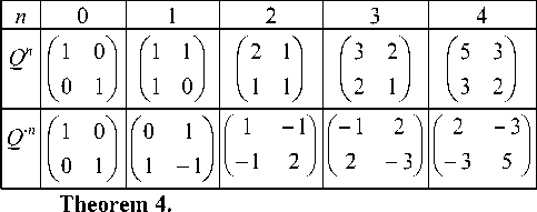
• Theorem 3.

Qn = Qn-1 + Qn-2.                                 (9)

Let us represent the expression of (9) in the form:

Qn-2= Qn - Qn-1.                                  (9-a)

The explicit forms of the matrices Q n ( n = 0, ± 1, ± 2, ± 3, .) obtained by means of the recurrent formulas of (9), (9-a) are given in Table 1.

F p (- p+ 1)= F p (- p + 2)=…= F p (0)= 0; F p (1) = 1(12) where n = 0, ± 1, ± 2, ± 3, ..

The numerical sequences generated with (11), (12) are called generalized Fibonacci numbers or p-Fibonacci numbers [15].

Note that p -Fibonacci numbers include in itself an infinite number of numerical sequences, in particular, the binary numbers for the case of p= 0 and the Fibonacci numbers for the case of p= 1.

In [16] the general theory of the Fibonacci matrices based on p -Fibonacci numbers was elaborated. A central notion of this theory is the notion of the Q p - matrix:

	l 1	1	0	0	0	0 ^	J
	0	0	1	0	0	0
	0	0	0	1	0	0	J
Qp =	0	0	0	: 0	: 1	0	JJ                   (13) JJ
	0	0	0	0	0	1	J
	1 1	0	0	0	0	0 J

where the index of p takes the values from the set {0, 1, 2, 3, …}.

Note that the Q p -matrix is the square (p+ 1) x ( p+ 1) matrix. It contains the p x p identity matrix bordered by the last row of 0’s and the first column, which consists of 0’s bordered by 1’s. For the cases of p = 0, 1, 2, 3 the Q_p -matrices have the following forms, respectively:

Q 0 = (1) ;

Q 1 =

= Q ;

^Q 2 = [ ⁰

l1

10 ^

0 0 J

	f 1	1	0	0 1
	0	0	1	0
Q 3 =	0	0	0	1
	1 1	0	0	0 J

Let us take without a proof [16] the following important theorems concerning to the Q_p -matrices.

	Theorem 5.
		' Fp ( - + 1)	Fp ( - )    ^	Fp ( - —	p + 1) '
		Fp ( - - p + 1)	Fp ( - - p ) ■■■	Fp ( - -	2 p + 1)
n Qp	=
		Fp ( - — 1)	Fp ( - — 2) ■	Fp ( - —	p — 1)
		ч    Fp ( - )	Fp ( - - 1) ■	Fp ( n	- p ) ,

The formula has a number of (14).

where Q is the Fibonacci Q- matrix of (2).

The abridged notation of the sums of (18) and (19) has the following form:

M = amam - 1... a 1 a о, a - 1 a _{- 2} ... a - m      ⁽²⁰⁾

Let us consider the representation of the 2 x 2 matrices in the code form of (20). It is clear that all powers of the Q - matrix are presented as the following code combinations:

Q ⁰= I = 1, 0; Q ¹= 10, 0; Q ²=100, 0; Q ^-1= 0, 1;

Q ^-2= 0, 01; Q ^-3= 0, 001; … .

Using (19) one may represent in the code form of (20) all the 2 x 2 matrices being some sums of the Q - matrix powers. For example the matrix

M = Q ³ + Q ¹ + Q ^-1 + Q ^-4 =

• Theorem 6.

Det Qnp= (-1)pn,(15)

where p = 0, 1, 2, 3, ... ; - = 0, ± 1, ± 2, ± 3, ... .

• Theorem 7.

П—Г>П - 1    n ^{- -} P ^{- 1}

Qp=Qp  + Qp     .(16)

• Theorem 8.

• 4.    Fibonacci matrix representation

m kk kk minm+

Qp x Qp = Qp x Qp = Qp

It is clear that Theorems 5, 6, 7 and 8 are the generalization of the well-known Theorems 1, 2, 3 and 4 for the classical Fibonacci Q -matrix.

Let us consider the binary positional presentation of the square ( p+ 1) x ( p+ 1) matrix in the following form:

M = Z aQ                    (18)

iip where ai is the binary numeral {0, 1}; Qip is the weight of i-th digit; Qp is the base of the number system (17); i = 0, ±1, ±2, ±3, . ; p = 1, 2, 3, . (the case of p = 0 is eliminated from consideration).

The formula of (18) gives an infinite number of the matrix representations of (18) because each number p generates its proper matrix representation of (18).

Note that the expression of (18) gives a certain class of the square ( p+ 1) x ( p+ 1) matrices, which could be represented in the form of (18). The matrices M, which could be represented (although potentially) in the form of (18) could be called the constructive matrices by analogy with the constructive numbers , which could be represented in the form of (1).

Let us consider now the partial case of (18) corresponding to p =1:

M ^«Qi                   (19)

6 1 1

1 5 ^J

-

+

- 3

- 3

is represented in the code form of (20) as the following:

M = 1010, 1001.

A special interest has the code representations of (20), which results from the following procedure. Let us consider the presentation of the identity matrix in the code form of (20):

M = I = Q ⁰ =       = 1, 00

1        01

In accordance with the property (9) we can represent the identity matrix of (21) in the following form:

I = Q ⁰ = Q ^-1 + Q ^-2                          (22)

In fact, using Table 1 we get:

0 1 1 f 1 -1 1 ( 10

+=

1 -1 ) ( -12 ) ( 0 1

Using (22) we can represent the identity matrix I in the code form:

I = 0,11

Adding 1 (the identity matrix I ) to the 0-th digit of (23) we get the following code combination:

M 2 =1,11

Using (9), we get the new representation of the matrix M 2 :

M 2 = 10, 01

The code combination of (25) corresponds to the sum

1    -2

M ₂ = Q ¹ + Q ²

1   1      1   -1       20

+       ==

1  0    -1  2      02

Then adding 1 (the identity matrix I ) to the 0^th digit of code combination (25) and using (9), we get the new code combination

M 3 = 100, 01,

which corresponds to the matrix

2    -2

m 3 = Q 2 + Q 2

2  1     1   -1      30

+         ==

1   1     -1   2       03

Continuing this process, i. e. adding 1 (the identity matrix I ) to the 0-th digit of the preceding code combination and using (9), we get the code representations of the following 2 x 2 matrices :

M 1	= I	0	0	0	0	1,	0	0	0	0
M 2	2 I	0	0	0	1	0,	0	1	0	0
M 3	3 I	0	0	1	0	0,	0	1	0	0
M 4	4 I	0	0	1	0	1,	0	1	0	0
M 5	5 I	0	1	0	0	0,	1	0	0	1
M 6	= 6 1 =	0	1	0	1	0,	0	0	0	1
M 7	= 7 1 =	1	0	0	0	0,	0	0	0	1
M 8	8 I	1	0	0	0	1,	0	0	0	1

b = F n + F p + … + F t , where n>p> …>t..

Next let us form from the number b two new numbers b + and b - according to the rule:

b + = F n+ 1 + F p+ 1 + … + F t+ 1 ;

b - = F n- 1 + F p-1 + … + F t-1 ;

Let us note that b = b + - b - . It follows from the definition (4) for the Fibonacci numbers.

Let us represent now the matrix of (27) as the sum of two matrices:

b   b     a-b 0

M =1 + l+l + I=

к b  b- J к 0     (a-b)-b- J

=(b +   b |+(a -b+    0 Yк b b -J к 0    a - b+J

Then the matrix

f b	b I
+
к b	b - J

can be represented as the following sum:

Continuing this process we could represent the matrix

^Fp+ 1

к

^Fn+ 1 F_n

F

Fn-1 J

+

Mn

n

0 n

= nl

Fp

77 к

F \

p-1 J

+ ... +

^{f F}t+1

к Ft

F7t I

^Ft- 1 J

in the form of (19). Thus the analyzed procedure of the 2x2 matrix coding permits getting the 2 x 2 matrices of the kind (26) only and hence the matrix of the kind of (26) are constructive one's regarding to the definition of (19).

Note there exists a one-to-one correspondence between the matrices of (26) regarding to the matrix representation of (19) and natural numbers regarding to Bergman's number system [3]. It means that we can use the isomorphism property for getting of code representation of the 2 x 2 matrices of the kind of (26). With this aim in view first we have to get the т -code of number n (the т -code is representation of natural number n in Bergman's number system [3]) . According to the isomorphism property the т -codes of numbers n coincide with the code representations (20) of the 2 x 2 matrices of the kind of (26).

Let us consider now the code representation of the 2 x 2 matrices of the following kind:

= Qn + Qp + … + Qt.

The code representation of the matrix of

a - b ₊

a - b+

= ( a - b₊ ) x I

can be got using the isomorphism between the matrices of the kind of (26) and natural numbers. For that it is necessary to get the т -code of the integer number of ( a -b₊ ). The latter representation togethe with the representation of (28) gives a possibility to represent the matrix of the kind of (27) in the form of (19).

For example let us consider the presentation of the matrix

R =

31 15 A

15 16 J

b a-b

where a and b are integers.

For getting the code representation of the matrix of (27) we will apply the following procedure. Let us represent the number b as some sum of the Fibonacci numbers, i. e.

in the form of (18). With this aim in view let us represent the number 15 as the sum of two Fibonacci numbers:

15 = F 7 + F 3 = 13 + 2.

Let us form now the numbers

15 + = F 8 + F 4 = 21 + 3 = 24

and

15- = F 6 + F 2 = 8 + 1 = 24

and represent the matrix R in the following form:

31  15 1   ( 21  13 1  ( 3  2 1  ( 70

—        ++

15  16 J  ( 13  8 J  (2  1J  (07

7    3         7    3     4-4

• —    Q ⁷ + Q ³ + 7 1 — Q ⁷ + Q ³ + (Q ⁴ + Q ⁴ ) — .

• —    Q ⁷ + Q ⁵ + Q ⁴

Thus the matrix R has the following code presentation:

31 15

R =          — 10100000,0001.

( 15 16 J

Let us consider now the matrix

„ (17 151 s.

( 15 2 J

This one could be represented as the sum:

21  131  (3  21  (-70

++—

13   8 J  ( 2  1 J  ( 0   - 7 J (29)

7   3      7   3/4-4 \

• —    Q ⁷ + Q ³ - 7 1 — Q ⁷ + Q ³ - Q ⁴ + Q ⁴ )

Using (9) we can represent the sum of (29) in the form:

7   3   4   -4    6   40-2

Q ⁷ + Q ³ - (Q ⁴ + Q ⁴ ) — Q ⁶ + Q ⁴ + Q ⁰ + Q ² +

• +    Q ⁴ + Q ⁵ - (Q ⁴ + Q ⁴ ) —

6    3    2    0    -2-5

• —    Q 6 + Q3 + Q2 + Q0 + Q 2 + Q

6    4    0    -2-5

• —    Q 6 + Q 4 + Q 0 + Q 2

Thus the matrix S has the following code representation:

17 15

s —          — 1010001 , 01001.

( 15 2 J

Above we considered in detail the code representations of the 2 x 2 matrices in the form of (19). The formula of (18) expands a class of Fibonacci matrix representations and is a source of new investigations in this field.

The identities of (9), (10) and their generalizations of (16), (17) form the basis of the Fibonacci matrix arithmetic.

Let us consider the simplest Fibonacci matrix arithmetic corresponding to the case of p= 1. Using (9) we can represent the sum of two matrix Q powers in the following form:

Qn + Qn = Qn + Qn-1 + Qn-2 = Qn+1 + Qn-2 . (30)

The identities of (30) underlie the matrix addition. Table 2 gives the addition rule of two single-digit 2 x 2 matrices.

Table 2

0	+	0 —	0
1	+	0 —	1
0	+	1 —	1
1	+	1 —	1	1	1 ( a )
1	+	1 —	10	0	1 ( b )

Using Table 2 for the addition of the matrices S+S = 2 S , we get the following code representation

2 S — 100001001 , 00101 —

83-3-5

• —    Q ⁸ + Q ³ + Q ³ + Q ⁵ — .

( 34 30 1    ( 17 15 1

• —          — 2 r

( 30 4 J    ( 15 2 J

The identity of (10) underlies the 2 x 2 matrix multiplication. Table 3 gives the rule of the matrix multiplication.

Table 3

0	x	0	— 0
0	x	1	— 0
1	x	0	— 0
1	x	1	— 1

Let us apply this rule for multiplication of the two matrices

M 2 = 10,01 and M 2 = 101,01

For multiplication let us represent these matrices in the form with the floating point:

M ₂ = 1001 x Q "² ; M 4 = 10101 x Q ².

After multiplication of the code combinations 1001 x 10101 we get the product

M ₂ x M 4 = 2I x 4 1 = 100010001 x Q ⁴ =

=10001, 0001= Q ⁴ + Q ⁰ + Q ^-4 =

5 31

3 2 J

+

- 3

- 3

8 I.

The positional matrix representations considered in the present article expand essentially the notion of the mathematical object positional representation. Unlike to the classical positional number systems where the numbers are the objects of code representation the objects of new positional presentation considered in the article are square matrices, which are more complicated mathematical objects in comparison to numbers. The bases of new positional representations are special matrices called the Fibonacci matrices.

It is shown in the article that only the matrices of the special kinds, so called constructive matrices, could be represented using new methods of matrix representation. This fact restricts practical applications of positional representations considered above. However, the

article puts forward a number of theoretical problems 6. concerning to matrix theory, in particular the problem to find a general method of Fibonacci matrix representa- 7. tion for arbitrary square matrix.

The American mathematician George Bergman who is the pioneer in non-traditional number systems 8. wrote in conclusion of his article [3]: "I do not know of any useful application for systems such as this, except as a mental exercise and pastime, though it may be of some service in algebraic number theory".                   9.

However progress of computer science refuted this pessimistic Bergman's statement. Just Bergman's number system and its generalization, the "Codes of the 10. Golden Ratios" [4], became of source of modern investigations in the field of the super-fast algorithms of digital signal processing [16].                                       11.

Probably the matrix representations based on the Fibonacci matrices could bring to new and unexpected applications to digital signal processing.                        12.