Matrix-based Kernel Method for Large-scale Data Set

Published Online December 2010 in MECS

In the field of machine learning, there are many successful methods to be used for feature extraction and dimension reduction. These methods are generally divided into two categories: linear methods and nonlinear methods. The commonly used linear methods include Principal component analysis (PCA) [1][2], Linear discriminate analysis (LDA) [3] and so on. Support Vector Machine (SVM) [4] and kernel principal component analysis (KPCA) [5] is the frequently used nonlinear methods. These methods have been used in many complex applications, such as face recognition, image compression, etc.

Principal component analysis (PCA) is a classical method for feature extraction and dimension reduction [6]. It uses the dimensions with larger variances and neglects the less important components. Linear discriminate analysis (LDA) is a classical technique for feature extraction and dimension reduction. It finds the subspace which maximizes the between-class and minimized the intra-class scatter matrices. Although these linear methods have been successfully used in many applications, it does not work well in nonlinear data distribution. Therefore, it is necessary to generalize the linear methods for the nonlinear structure.

Vapnik et al. [4] firstly introduced kernel method [7] into Support Vector Machine. After that, it has successfully generalized to kernel principal component analysis, Generalized discriminant analysis [8] and other algorithms. Its main idea is to map the data set from the input space into high-dimensional feature space. Thus, the nonlinear components can be extracted using the traditional linear algorithm in feature space. The kernel trick is used to calculate the inner product between data set without knowing the explicit mapping function. These nonlinear methods have been used in classification, regression and supervising learning [9][10][11], etc.

In the computation process, many kernel methods need to compute the kernel matrix for all samples. For example, SVM uses all the training samples to learn hyperplane to maximize the separating margin. It needs to solve the quadratic programming (QP) problems, which time and space complexity is O ( m ³) and O ( m ²) respectively, where m is the number of data samples. The standard KPCA generally needs to eigen-decompose the kernel matrix (called Gram matrix) , which is acquired using the kernel function. It must firstly store the kernel matrix of all data, which takes the space complexity of ο ( m ² ) . In addition, it needs the time complexity of ο ( m ³ ) to extract the kernel principal components. But traditional kernel function is based on the inner product of data vectors, the size of kernel matrix scales with the number of data set. When faced with the large-scale data set, it is infeasible to store and compute the kernel matrix because of the limited storage capacity. However, the evergrowing large-scale data set needs to be processed in many applications, such as data mining, network data detection and video retrieval. Consequently, some approaches must be adopted to account for the inconvenience.

In order to solve the problem of the large-scale data set, some methods have been proposed to reduce the time and space complexities. In general, these approaches are classified into two categories: the sampling and nonsampling based approaches.

For the sampling based approaches, Zheng [12] proposed to partition the data set into several small-scale data sets and handle them, respectively. Some representative data [13] are chosen to approximate the original data set. Some approximation algorithms [14][15][16][17][18] are also proposed to extract the nonlinear components. The major difference between these methods lies in the sampling way. One disadvantage is that these methods will lose some information in the sampling process. Aside from that, it is time-consuming to search for the representative data.

In this paper, we propose a new framework, matrixbased kernel methods, which can effectively solve the problem of large-scale data set. We have given elementary application on KPCA [23] and SVM [24]. In this paper, we will give further demonstration and discussion. The core idea of matrix-based kernel methods is firstly to divide the large scale data set into small subsets, each of which can produce the 1-order and 2-order statistical quantity (mean and autocorrelation matrix). For the 1-order statistical quantity, the traditional kernel method can be used to compute the kernel matrix. Because the 2-order statistical quantity is a matrix, we proposed a novel polynomial-matrix kernel function to compute the similarity between 2-order statistical quantities. Because the number of subsets is less than the number of samples, the size of kernel matrix can be greatly reduced. The small size of kernel matrix makes the computation and storage of large-scale data set possible. The effectiveness of the proposed method is demonstrated by the experimental results on the artificial and real data set.

The rest of this paper is organized as follows: section II gives reviews of kernel methods. Section III describes the proposed algorithm in detail. The experimental evaluation of the proposed method is given in the section IV. Finally we conclude with a discussion. .

• II.    REVIEW OF KERNEL METHODS

Let X = ( X₁,X 2 ,..., X m ) be the data matrix in input space, where X i , i = 1,2,..., m , is a n-dimensional vector and m is the number of data samples. There exists a mapping function ф , which projects the data into highdimensional (even infinite dimensional) Reproducing Kernel Hibert Space (RKHS).

• ф :      ^ n ^ F

X a ^{ф (} x i )           (i)

Using mapping function ф , we can get the projected data set Ф(X) = (ф(X1),ф(X2),...,ф(Xm)) in feature space. In practice, the mapping function ф needs not to be known explicitly but performed implicitly via kernel trick. A positive definite kernel function k(.,.) is used to calculate the dot product between mapped sample vectors, where     k(.,.)     is given by

к (.,.) = k ( X_i , X j ) = ф ( X i ) T ф (X j ) . The polynomial and Gaussian kernel are two widely used kernel function, given by:

• ^{к (}.,.) = ^{ф ( X}i ) T ^{ф ( X}j ) = ⁽ X T^ ) ^d

T                      || X i — X j ||

• ^K C,.) = ^{ф (} X ) ^{ф ( X}j ) = exp⁽-- _Q 2   )

• ^{1                                   2 c}         (2)

Where d is the degree of the polynomial kernel function and C T is the width parameter of the Gaussian kernel function.

Many algorithms based on kernel method were proposed to treat with the nonlinear datum. We only give some derivation of KPCA and other algorithms are similar.

In mapping feature space, the covariance matrix is given as follows:

m

C = —Z ^{ф ( X}i ) ^{Т ф ( X}i )

^m i = i                                 (3)

It accords with the following equation:

C v = Av                  (4)

Where V and A are corresponding eigenvector and eigenvalue of covariance matrix. It is an intractable task to solve the eigen-equation directly, which can be overcome via kernel trick. The solution V can be expanded using all the mapping sample vectors in the data set Ф(X) = (ф(^),ф(X2),...,ф(Xm)) as:

m

• ^v = Z “ i ^v ^Xi )

i = 1                                            (5)

By substituting Eq.3, Eq.5 into Eq.4, we can get the following formula:

K a = m Aa                (6)

Where ^a is span coefficient, ^K is Gram matrix denoted as K = Ф ( X ) T Ф ( X ) = ( k j )_{1 S} i , j _{s m} . The entry of Gram matrix is k ij = k ( X i , X j ) . It is proven [25] that the Gram matrix is positive semi-definite. To compute the kernel principal components, the traditional method is to diagonalizable Gram matrix K using eigen-decomposition technique.

Once the eigenvector a has been achieved, we can achieve the kernel principal components V using Eq.5. For a test sample x , the nonlinear feature is given:

m

( ν , φ ( x )) = ∑ α _i ( φ ( x_i ) ⋅ φ ( x ))

i = 1

m

= ∑ α _ik ( x_i , x )

i = 1                                   (7)

kernel method is based on vector, the 2-order statistical quantity is a matrix. We must find some way of

approaching the problem.

In the process of whole derivation, it is assumed that the data have zero mean, if it is not, we can get the centering matrix K = K - 1 _mK - K 1 _m + 1 _mK 1 _m , ¹

where 1 _m = () _{m × m} .

m

In this circumstance, we can treat them as the special computational units in input space. The data autocorrelation matrix can also be considered as generalized form of data vector. It is shown [6] that the autocorrelation matrix contains the statistical information between samples.

Thus, the special computational unit can be projected into high-dimensional (even infinite dimensional) Reproducing Kernel Hibert Space (RKHS) using a mapping function φ .

III. THE PROPOSED ALGORITHM

The data set X = ( x ₁, x ₂,..., x_m ) is firstly divided into M subsets X_i ( i = 1,..., M ) , each of which consists of about k = m / M . Without loss of generality, it is denoted:

φ :       ℜ ^{n × n} → F

Z , a ^ ( 1 , )

After having projected into feature space, the data set can be represented as Φ ( ∑ ) = ( φ ( ∑ ₁), φ ( ∑ ₂),..., φ ( ∑ _M )) .

M

Accordingly, X = U X i = ( X i , X 2 ,..., X m ) .

i = 1

A. Computing 1-order statistical quantity

First, we compute 1-order statistical quantity (mean) for each subset. It is given as follows:

center

1 ^k

⁼ k ^∑ i = 1 ^{x i}

center

, X_M

C. A novel polynomial-matrix kernel function

In this situation, we also need not know the mapping function explicitly, but perform it via kernel trick. According to the Eq.2, traditional kernel function is based on the inner product of data vector. Because the special computational unit is now based on matrix, the kernel function cannot be used. In order to compute the similarity between the mapping computational units in feature space, a positive definite kernel function needs to be denoted .

Considering to characteristic of polynomial kernel function, a novel polynomial-matrix kernel function is denoted as:

1 m - ( M - 1) k

m

∑ x i

i = ( M - 1) k + 1

Having computing mean of each subset, the 1-order statistical quantity is still a vector. The standard kernel method can be used to map it to high dimensional space.

k (.,.) = k ( ∑ _i , ∑ _j )

= №)№ , )) = || Z _; . *z _y ii D

B. Computing the autocorrelation matrix of subset

Similarly, 2-order statistical quantity (autocorrelation matrix) for each subset can be computed. The autocorrelation matrix can be defined as follows:

∑ ₁ = X ₁ X ₁ ^T , ∑ ₂ = X ₂ X ₂

T

T

M ⁼ MM

w here || . || _B = || (.).^1/2 || _F ( || . || _F is the f robenius norm of matrix), . ∗ denotes the component-wise multiplication of matrices, .^1/2 means the componentwise square roots of matrices, and D is the degree of the polynomial-matrix kernel function. Now, we will investigate if the polynomial-matrix kernel function has some relationship with the polynomial kernel one.

The data set X = ( X ₁, X ₂,..., X_M ) is then

transformed into ∑= ( ∑ ₁, ∑ ₂,..., ∑ _M ) , where ∑ _i is n × n autocorrelation matrix. Because the traditional

Theorem: When each subset has one sample, the polynomial kernel function based on the data vector equals to twice of the polynomial-matrix one based on the autocorrelation matrix. That means the degree d is the twice of the degree D.

Proof:

When each subset contains one sample, the autocorrelation matrix Z i = X^X T . Using the polynomial-matrix kernel function, it follows:

k ( Z i , z j ) = || z i . *z , ii D

TT ^D

= 11 ^ . * x j x j  II B

i 1 x in

^Xj 1 ^Xjn )

( N ⁺ + N ) x ( N ⁺ + N ) by the novel polynomialmatrix kernel function. The small size of kernel matrix makes the computation and storage possible. Thus, the general SVM method can be used except that the vector was substituted for matrix.

In the case of training case, all the training clusters meet the following constraints:

y( мф (X_t ) + b ) >  1 - 6 , i = 1,2, L ,( N ⁺ + N -) ₍₁₃₎ where mapping function ф projects the matrix subset into high-dimensional (even infinite dimensional) Reproducing Kernel Hibert Space (RKHS).

Similarly to the SVM, the SMM also learns hyperplane to maximize the separating margin between the positive and negative subset. By introducing the regularization term, the cost function can be transformed into minimize the VC bound ：

= (( ^Xi 1 ^Xj 1

+ x i 1 x i 2 x j 1 x j 2 + ,

in jn

2₎₎ D

n

= ((Z x^x, )2)D k=1

= ( x T X j ) 2 ^D = k ( X i , X j )^{2 D} = k ( X i , X j ) ^d

, and the theorem is derived.

In other words, the polynomial kernel function is the extreme case of the polynomial-matrix one, when each subset comprises only one sample. The theorem also shows the kernel matrix computed using two different kernel functions is same at this time, which can give the same classified result when used in the kernel method.

We have given the matrix-based kernel method. Now, we will give specific application for some kernel-based algorithms ---support vector machine and kernel principal component analysis. Other kernel algorithms can be derived similarly.

1 _T min — to to

™ 2

( N + + N ^- )

+ C z 6

i = 1

The dual problem can be transformed like the SVM, which can be given as:

( N + + N ^- )       1 ( N + + N )( N + + N ^- )

max Z ^a i ^- Z Z y_iУ j «a j ^{ф (X}_i)^{T ф (}X )

i = 1             ² i = 1        i = 1

s . t .

1 <  a i < C , i = 1, l , k

( N ⁺+ N ^- )

Z a y i = 0

i = 1

D. Support Matrix Machine (SMM)

Let X ⁺ = ( X , X ₉,..., X ₊ ) and 12 _m

X = (X + ,X + ,...,X + -) be the positive and m + +1 m+ +2 m + + m negative samples, respectively, where Xi, i = 1, 2,l, m + + m , is a n-dimensional vector and m+, m is the number of positive and negative samples separately. The label yi corresponding to sample xi lies in {1,-1}. For the proposed method, positive and negative samples are firstly clustered using Kmeans Algorithm, respectively. The N+ positive and N-negative training clusters can be obtained.

Because the data set is divided into many subsets in positive and negative samples, the number of subsets is less than the number of original data set. As a result, the large-scale data set is compressed by down-sampling the data using the matrix of each subset. In this situation, the size of kernel matrix can be greatly reduced from ( m ⁺ + m ^- ) x ( m ⁺ + m ^- ) to

Using the quadratic programming (QP) solver, the parameter a i , i = 1, l , k can be easily obtained.

In the case of testing case, for a test sample x, its autocorrelation matrix Z _X = XX T and following decision function can be used to predict it:

( N ⁺+ N ^- )

f ^{( x} ) = sgn⁽ Z а-у - ^{ф ( X}- ) ^{т ф ( X} ))

i = 1                                        (15)

From above derivation, it shows that the proposed SMM has the same framework as the SVM except that the vector is replaced with matrix.

E. Kernel Principal Component Analysis based on 2-order statistical quantity

Because the data set is divided into many subsets, the number of subsets is less than the number of original data set. As a result, the large-scale data set is compressed by down-sampling the data using the matrix of each subset. In this situation, the size of kernel matrix can be greatly reduced from m x m to M x M by the novel polynomial-matrix kernel function. Thus, the small size

of kernel matrix makes the computation and storage possible .

Currently, the mapped data set is Φ ( ∑ ) = ( φ ( ∑ ₁), φ ( ∑ ₂),..., φ ( ∑ _M )) in feature space. The similar Equation for nonlinear component analysis can be derived. The covariance matrix is given as follows:

M

C = ¹ ∑ φ ( ∑ ) ^T φ ( ∑ )

M i = 1    ⁱⁱ       (16)

It also accords with the eigen-equation:

C ^{ν = λν}              (17)

But the eigenvector is now expanded using the linear sum of projected matrix in Φ ( ∑ ) = ( φ ( ∑ ₁), φ ( ∑ ₂),..., φ ( ∑ _M )) as:

ν = ∑ ^M α i φ ( ∑ i )

^{i = 1}                                  (18)

Therefore, the centering kernel matrix is K=K-1MK-K1M+1MK1M, where

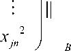
Figure 1. Learning result on the 2-D toy problem obtained from the standard SVM (upper left) and SMM (upper right, lower left, lower right)

By substituting Eq.14, Eq.16 into Eq.15, we can get

the following formula:

K α = m λα

1 M = (¹) M M

M × M

Where α is span coefficient, K is Gram matrix denoted as K = Φ ( ∑ ) ^T Φ ( ∑ ) = ( k_ij )_{1 ≤ i , j ≤ M} . The entry of Gram matrix is k_ij = k ( ∑ _i , ∑ _j ) . After having got the eigenvector α , the kernel principal components ν can be achieved using Eq.16.

For a test sample x , its autocorrelation matrix is ∑ _x = xx^T . The nonlinear feature is then given:

MM ( ν , φ ( ∑ _x )) = ∑ α _i ( φ ( ∑ _i ) ⋅ φ ( ∑ _x )) = ∑ α _ik ( ∑ _i , ∑ _x ) i = 1                                        i = 1

In the process of whole derivation, it is assumed that the special computational unit, autocorrelation matrix of data subset, has zero mean; otherwise, it is easy to derive the centering kernel matrix:

k%(∑i,∑j)=||(∑i-1∑).∗(∑j-1∑)||CD ij iMjMC

= ||( ∑ . ∗∑- ¹ ∑ . ∗∑- ¹ ∑ . ∗∑ ⁱⁱMⁱ Mⁱ

+ _M ¹ 2 ∑∗∑ )|| C ^D

= ( K - 1 K - K 1 + 1 K 1)

MMMMij

The computation process of proposed Kernel Principal Component Analysis based on 2-order statistical quantity is shown in Algorithm 1, Kernel Principal Component Analysis based on 1-order statistical quantity is identical to the traditional KPCA.

IV. experiment

To demonstrate the effectiveness of the proposed kernel methods, we do some experiments using support matrix machine and kernel principal component analysis for large scale data set.

• A.    Experiment using support matrix machine

Firstly, we perform the experiments on twodimensional toy problem using the standard SVM and the proposed SMM method, respectively. In addition, we use USPS data set to validate the feasibility of SMM. The polynomial kernel k ( x , y ) = ( x^T y ) ^d (where d is the degree) is used in standard SVM. The polynomial-matrix kernel function k ( ∑ _i , ∑ _j ) = || ∑ _i . ∗∑ _j || _C ^D (where D is the degree) is used in SMM. The sample of cluster in the Kmeans algorithm is adjusted according to the training samples.

Toy examples:

We firstly use 2-dimensional toy problem to demonstrate the effectiveness of SMM. 500 positive and 500 negative samples are generated, where follows a Gaussian distributions. In the SMM, the data set of each class is divided into 150, 250,500 subsets, respectively. The degree d and D of two kernel function equal to 2 and 1, respectively.

The experiment results are given in Fig. I. The support vectors were labeled in red bold. From the result, SMM can get almost similar performance with the standard SVM. The result shows the effectiveness of SMM, which can successfully learn hyper plane to maximize the separating margin.

USPS examples:

We also test the proposed method on real-world data. The US postal Service (USPS) data set {Available at

TABLE I.

SVM SMM with different k the size of samples in each class K=400 K=500 Error Rate(%) 4.68 4.68 4.73 4.78 } is 256-dimensional handwritten digits '0'--'9'. It consists of 7291 training samples and 2007 testing samples. It is known the recognition rate for the dataset is only 2.5% for human [26]. In order to test the proposed method, a preprocessing step was firstly used with a Gaussian kernel with width 0.75 to smooth the image. For each method, we use the average result of 45 one-against-one classifiers. The degree d and D of the kernel function in two methods equal to 4 and 2, respectively.

Table I gives the average testing errors obtained by the standard SVM and the proposed method. In the proposed SMM, the number of cluster in each class was set to 400, 500 and the size of the samples in each class, respectively. When the number of cluster in each class was equal to the size of the samples in each class, which means the class is still original dataset. Although the dataset is not clustered at this time, matrix is still used to replace vector in the computation process. According to the above theorem, the two methods can get the same result, which can be found from the table. In addition, it also shows that the performance based on matrix of cluster is comparable to standard SVM.

• B.    Experiment using Kernel Principal Component

Analysis

To demonstrate the effectiveness of the proposed methods, we perform the experiments on twodimensional toy problem using the standard KPCA (using the original Matlab source code [5] available at and the proposed methods, respectively. In addition, we use USPS data set to validate the feasibility of proposed methods when standard eigen-decomposition technique cannot be applied. In order to differentiate from the standard KPCA, we abbreviate the method 1order-KPCA, which means Kernel Principal Component Analysis based on 1-order statistical quantity and shorten the method 2order-KPCA, which means Kernel Principal Component Analysis based on 2-order statistical quantity. The polynomial kernel k(X, y) = (XTy)d (where d is the degree) is used in standard KPCA and 1order-KPCA. The polynomial-matrix kernel function

Figure 2. Contour image of first 3 principal components obtained from standard KPCA (the first row), 1order-KPCA (the second row) and 2order-KPCA(the third row).

k ( X i , X j ) = || X i . *X j || D (where D is the degree) is used in 2order-KPCA

Toy examples:

We firstly use 2-dimensional toy problem to demonstrate the effectiveness of proposed methods. The 200 2-dimensional data samples are generated, where x-values are uniformly distributed in [-1,1] and y-values are given by y = X 2 + П ( П is the normal noise with standard deviation 0.2). In the 1order-KPCA and 2order-KPCA, the data set is divided into 100 subsets, each of which contains 2 samples. The degree d and D for two kernel functions equal to 2 and 1, respectively.

The 1-order statistical quantity and 2-order statistical quantity was firstly computed. The experiment results are given in Fig.2. It gives contour lines of constant value of the first 3 principal components, where the gray values represent the feature value. From the result, the 1order-KPCA and 2order-KPCA can get almost similar performance with the standard KPCA. The result shows the effectiveness of proposed methods, which can successfully extract the nonlinear components.

USPS examples:

Firstly, we randomly select 3000 training samples to extract the nonlinear feature. In the proposed methods, we divide 3000 training samples into some subsets with different size ( 1 <  k <  5 ) in each subset. For each k, 10 independent runs are performed, where the data samples are randomly reordered. The classified results of 2007 testing samples are averaged.

TABLE II.

E rror rate of 2007 testing sample using proposed methods ( having degree d =1 and different sample numbers k in each SUBSET ) AND THE STANDARD KPCA ( HAVING DEGREE d =2) WITH 3000 TRAINING SAMPLES .

Number of components	KPCA	1order-KPCA with d=2
		K=1	K=2	K=3	K=4	K=5
32	7.17	7.17	6.88	7.13	7.08	7.22
64	6.98	6.98	6.98	7.08	7.13	7.13
128	7.17	7.17	7.47	7.22	7.47	7.52
256	7.22	7.22	6.93	7.13	7.22	7.13
512	7.42	7.42	7.32	7.13	7.21	7.03

(a). Result of 1order-KPCA

Number of components	KPCA	2order-KPCA with D=1
		K=1	K=2	K=3	K=4	K=5
32	7.17	7.17	7.27	7.03	7.17	7.42
64	6.98	6.98	6.98	6.93	6.78	6.78
128	7.17	7.17	7.37	6.88	7.08	7.03
256	7.22	7.22	7.32	7.03	7.22	6.93
512	7.42	7.42	7.27	7.47	7.32	7.42

(b). Result of 2order-KPCA

Table ii ~~Table iv gives the error rate of testing sample using standard KPCA and proposed methods with different number samples in each subset. Table ii, Table iii, and Table iv are the results of the polynomial-matrix kernel function under degree D = 1,1.5 and 2 for 2order-KPCA, respectively. It also gives the corresponding result of the polynomial kernel function under degree d = 2,3 and 4 for standard KPCA and 1order-KPCA, respectively. According to the aforementioned theorem, when each subset has one sample, the polynomial kernel function based on the data vector equals to twice of the polynomial-matrix one based on the matrix. In this situation, the result of 1order-KPCA and 2order-KPCA should equal to the result of the standard KPCA (one sample in each subset), which can be found in each Table. It also shows 1order-KPCA and 2order-KPCA with different number samples in each subset could generally achieve competitively classified result than the standard KPCA. The reason may be that the mean and autocorrelation matrix contains the statistical information between samples in each subset. In addition, the computation instability for the small size kernel matrix can be greatly reduced when performing its eigen-decomposition. To visualize the result more clear, we plot the recognize rate under different number of kernel principal components in Fig.3~~Fig5.

In addition, we also use all the training samples to extract the nonlinear feature. Because the size of Gram matrix is 7291 x 7291 , it is impossible for standard KPCA algorithm to run in the normal hardware. Using the proposed methods, we firstly divide 7291 training samples into 1216 subsets, each of which consists of 6 samples (The last subset contains only 1 sample). Table 5 is the result of proposed method with 6 samples in each subset trained with all training samples. Here, the size of kernel matrix drops from 7291 x 7291 to 1216 x 1216 , which can be easily stored and computed. As shown in Table Ⅴ , it can also be seen that 1order-KPCA and 2order-KPCA can achieve the right classified performance even the eigen-decomposition technique cannot work out when faced with large-scale data set.

The result shows that the proposed method is more effective and efficient than standard KPCA.

IV. ConclusioN

In this paper, an efficient matrix-based kernel method for large-scale data set is proposed. The method firstly divides the large scale data set into small subsets, each of which can produce autocorrelation matrix. Then the autocorrelation matrix can be treated as special computational units. The similarity between matrices can be computed using a novel polynomial-matrix kernel function. It can greatly reduce the size of kernel matrix, which can effectively solve the large scale problem.

Compared to other related methods, the proposed method is different in the following aspects: (a). the proposed method uses the matrix, while other methods use data vector, as the computational unit in data space. (b). the autocorrelation matrix contains the correlation information of sample subset, which can help the improvement of performance. (c). the proposed method can be easily implemented; while many other methods are more complicated.

We only consider the polynomial-matrix kernel function in the whole process. We will investigate other kernel function based on matrix. In addition, the optimal sample number in each subset deserves further study in our future work

Acknowledgment

This work was supported in part by Doctor Fund of Henan University of Technology under contract 2009BS013, and Innovation Scientists and Technicians Troop Construction Projects of Henan Province under contract 094200510009.