Modeling and forecasting public debt in South Africa

Business success and government’s investment policy as well as macroeconomic policy are influenced by the accuracy of public debt forecasts. Public debt is sometimes referred to as government debt, it represents the total outstanding debt of a country’s central government. It is often expressed as a ratio of Gross Domestic Product (GDP). It is understood that public debt is a crucial source of resources for a government to finance public spending and close the gaps in the budget. Therefore, public debt as a percentage of GDP is usually used as an indicator of the ability of a government to meet its future obligations. According to (Burriel et al. 2020), debt is integral to the functioning of a market economy. The literature has indicated that there are certain cost and benefits of debt for any economy. On the note of benefits, they have indicated the following factors, firstly; public debt plays an important role for the functioning of the financial system and the transmission of monetary policy. Secondly, public debt can have direct effects on welfare as long as it offers a safe asset for insurance against cumulative risks. On the other hand, high debt burdens can ultimately impede long-term growth. (Checherita-Westphal et al., 2014) explained that this is evident in the case when debt is contracted to finance unproductive expenses or beyond optimal levels of public capital stock.

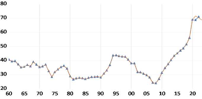
According to (Were, Mollel, 2020) the median level of public debt in sub-Saharan Africa (SSA) as of the end of 2017 exceeded 50% of GDP. The financial crisis that erupted in mid-2008 led to an explosion of public debt in many advanced and developing economies (Cecchetti et al., 2010). One of the reasons postulated in (Balassone et al, 2011) is that growing public debt in an economy is linked to the lack of accumulated saving and low investment levels. Furthermore, the work (Schularick, 2012) indicated that due to South African context the financial unsustainable public-owned institutions have exacerbated public debt. The deterioration in South African public debt it has been observed over the years now. Figure 1 presents the ratio of total public debt to GDP in the period from 1960 to 2022.

Figure 1. Total public debt as a percentage of GDP for 1960–2022

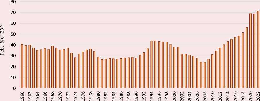
Years

Source: own compilation using data from SARB

Figure 1 illustrates that total public debt as a percentage of GDP from 1960 to 1978 was in a cyclical pattern, and its peak during the cycle was 40% and the lowest debt during the time was 28.4%. In the year 1980 to 1990 total debt was at average around 29.3 % of GDP, this seems to be the period in which debt was at its lowest. In the year 1998 total debt was 42.7% of GDP and was significantly reduced to 24.0% of GDP in 2008. According to (Mahadea, 1998) this achievement of reduction in public debt can be plausibly argued that this is the success of Growth, Employment and Redistribution (GEAR) policy. However, in 2008 public debt as a percentage of GDP grew exponentially from 24.0% to 71.1% in 2022. This growing sign of public debt is really a concern since government finances were already on a deteriorating trajectory.

The main purpose of this paper is to contribute to the debate about modeling and forecasting of public debt in South Africa through the lens of ARIMA models. In some instances, it can be argued in the literature that there are some factors that can be used to explain the behavior of public debt according to (Zhuravka et al., 2019; Munir, Mehmood, 2018). However, it should be mentioned that such approach may sometimes fall to a trap of selecting inappropriate and insignificant variables in modeling public debt. It is, therefore, the interest of the current study and more appropriate to adopt a more robust univariate time series technique such as ARIMA.

Public debt is one of the critical components of fiscal policy for the development of the economy and yet accumulating stock of debt remains a serious problem in South Africa. This is exacerbated by faster accumulation of debt compared to slower service of debt. For any economy, especially emerging country like South Africa, public debt forecasting is vital for proper debt management. It can be mentioned that an accurate and reliable modeling and forecasting of public debt in South

Africa is certainly important to avoid putting the country into unsustainable debt situation. Therefore, the objectives of this paper are as follows: 1) to analyze public debt trends in South Africa over the study period; 2) to develop a reliable public debt forecasting model for South Africa based on the Box – Jenkins method; 3) to forecast public debt in South Africa for 2021–2023.

Literature review

Increasing public debt is one of the problematic macroeconomic variables that occupy a central place in public debt management of most economies. This is so because it is mostly used as one of the fiscal indicators in the country’s public finances. According to (Mellet, 2014), one of the main instruments of fiscal policy is the budget which is the vehicle to change any of fiscal elements to ultimately change the spending behavior of the country inhabitants. Cecchetti, Mohanty and Zampolli (Cecchetti et al., 2010) explained further that when a country starts from an already high level of government debt, the probability that a given shock will trigger unstable debt dynamics is higher. This risk is amplified when public debt is already on a steep upward trajectory, as it is currently being observed in several countries. One of the arguments claimed by Minakir and Leonov (Minakir, Leonov, 2019) in Russia is that large of part of public debt it can be attributed by the fact that large proportion of debt is the implementation of social welfare against capital investment activities. The study (Dumitrescua, 2014) provided the framework for the analysis of the public debt-GDP ratio evolution in Romania in the period 2002–2012. The study found that Romania’s position regarding government debt level is apparently comfortable, the projected level for the end of 2013 being of 37.85% of GDP. Nikoloski and Nedanovski (Nikoloski, Nedanovski, 2017) studied the dynamics of government debt for the Republic of Macedonia and the possibility of its projection in the near future. The found that in considering the recent status and the impact of a range of political and socio-economic factors in the country, the estimate of the level of government debt in 2017 is approximately 40% of GDP.

Zaja, Krzic and Habek (Zaja et al., 2018) engaged in a study to forecast fiscal variables in selected European economies (Portugal, Ireland, Greece, Spain, and the Republic of Croatia) using least absolute deviation method. The study found that based on the conducted analysis of the fiscal variables among the countries, it can be said that balanced budgets have virtually disappeared, and public debt has prevailed. Zhuravka, Filatova, and Aiyedogbon (Zhuravka et al., 2019) explored the theoretical and practical aspects of forecasting public debt in Ukraine. Their paper concluded that ARIMA model (1, 1, 3) is the most accurate in describing the trend of public debt dynamics and provides the highest accuracy for further forecasting. The work (Were, Mollel, 2020) provides an analysis of public debt and debt sustainability in Tanzania, focusing on external debt. The paper provides an analysis of public debt and debt sustainability, and it was found that external debt accounts for over 70% of public debt in Tanzania. Rahman and Pujiati (Rahman, Pujiati, 2021) collaborated in research paper to forecast the value of Indonesian government foreign debt over the next five years from 2020 to 2024. The study concluded that the value of government foreign debt is predicted to keep increasing from 2020 to 2024.

In South African context the work of Calitz, Siebrits and Stuart (Calitz et al., 2016) studied the accuracy of fiscal projections. The paper strengthens the argument that the government should continue to strengthen its fiscal framework by adopting expenditure ceilings for the main budget and by expanding the availability of information on aspects of fiscal policy. It can be said that much of literature in South African context is between public debt and economic growth (see, for example: Baaziz et al., 2015; Mhlaba, Phiri, 2017).

What is absent in the preceded mentioned studies is an attempt to model total public debt in South Africa using ARIMA models. However, this leaves a knowledge gap of existing studies based on univariate ARIMA modeling. For knowledge contribution purpose, the study forecast public debt for South Africa using time series for time horizon of 1960–2022. The motivation to embark upon such a study is quite simple. Applying a time series (total public debt) forecast gives us the opportunity to extract information from the past. The assumption is that past trend will follow in future which gives us the evolution of future scenario based on the past information. In view of this, the objective of this study is to model total public debt in South Africa by making use of ARIMA model.

Data and research method

This paper makes use of the secondary data which is freely downloaded from a reliable source which is South African Reserve Bank (SARB). The variable in use is total loan debt of national government: total gross loan debt as percentage of GDP. The dataset was collected for the period 1960 to 2022. This time span is not motivated than just to explore the available data.

The Box – Jenkins method was proposed by George Box and Gwilym Jenkins in their seminal 1970 textbook Time Series Analysis. The method starts with the assumption that the process that generated the time series can be approximated using an autoregressive moving average (ARMA) model if it does not contain a unit root or an autoregressive integrated moving average (ARIMA) model if it is nonstationary. The paper applies the ARIMA model which uses values of government debt that are affected by the values of government debt in the past. The general expression of the Box – Jenkins model it is formed on the bases of two components which is the autoregressive (AR) and moving average (MA). Where the AR are models in which the value of a variable in one period is related to its values in previous periods, and MA models account for the possibility of a relationship between a variable and the residuals from previous periods. Therefore, ARMA can be expressed as follows:

DBTP_t = a + P i DBTP t-i + $₂DBTP_t-2 + ... +

, (1)

• + P_pDBTP_t — _p + (p i e — + (р₂е — + ... + (p_qe_t — _q

where DBTP _t — public debt that depends only on its own lags. That is, GBTP _t is a function of the “lags of GBTP _t- p ” Likewise, a pure Moving Average (MA only) model is one where DBTP _t depends only on the lagged forecast errors p _q e _t-q . Where the error terms are the errors of the autoregressive models of the respective lags. The Box – Jenkins mode comprises four stages.

• 1)    Model identification: this step involves selecting the most appropriate lags for the AR and

MA parts, as well as determining if the GBTP requires first-differencing to induce stationarity. The autocorrelation (ACF) and partial autocorrelation function (PACF) are used to identify the best model to estimate GBTP. (Information criteria can also be used).

• 2)    Model estimation: this step usually involves the use of a least squares’ estimation process by estimating GBTP with its past values and its errors.

• 3)    Diagnostic checking of the model: this step usually is the test for autocorrelation. Diagnostic testing of the model consists of normality test (Jarque – Bera) test, Inverse roots of AR and autocorrelation test. This involves post estimation tests to ascertain that the best GBTP model selected is appropriate for forecasting.

  
  
  
  
  
  

• 4)    Model forecasting: one of the main goals of the analysis on time series models is forecasting. The ARIMA models are particularly useful for forecasting due to the use of lagged variables. At this stage the paper will provide the forecasted values of GBTP and compare them with actual values to evaluate the forecasted values.

Empirical results

This section of the study provides the results on analysis of government debt in South Africa.

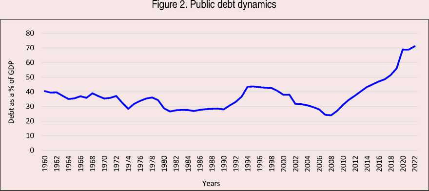
An annual time series of public debt for the period of 1960 to 2022 is presented in Figure 2.

It can be observed that the variable is non-stationary at levels since there are some trends showing upward trend especially from 2008 to 2022. However, the variable shows some stationarity after it has been first differenced where its mean, and its variance is reverting around zero.

The test was carried out first with an intercept only, then a trend and intercept. In each case the Ho: p = 0 was not rejected at the 5% significant levels given the ADF test value of -0.938 in levels. However, it can be observed that at first difference the ADF t-statistics of -4.931 is significant at 5% with a p-value of 0.000. The similar results can also be observed on the Phillips – Perron results, and it can be concluded that the variable is stationary after the first difference.

Model identification results

In estimating the ARMA the first step is to consider the graphs of the partial autocorrelation function and autocorrelation of a series of public debt for South Africa (Fig. 3, 4) to determine the general specification of the future ARIMA model and the number of lags for each component. The correlogram graphs are analyzed based on the key properties of the graphs of ACF and PACF functions for ARMA processes.

Table 1. Descriptive results of the study

Variable	DBTP
Obs.	63
Mean	36.95
Std. dev.	10.00
Min	24.00
Max	71.10

Table 2. Augmented Dickey – Fuller test and the Phillips – Perron test for DBTP variable

	Intercept only
	ADF results	PP results
Level s	-0.938 (0.769)	-0.497 (0.884)
First difference	-4.931 (0.000)***	-4.931 (0.000)***
	Trend & intercept
Levels	-1.375 (0.858)	-0.952 (0.942)
First difference	-5.217 (0.000)***	-5.247 (0.000)

• Figure 3.    Total public debt as a percentage of GDP at levels

  Autocorrelation Partial correlation							АС	PАС	Q-Stat	Prob
  1						1	0.88..	0.88.	.. 51.28..	. 7.97...
  1			■		1	2	0.72..	-0.2.	.. 86.70..	. 1.48...
  1				■	1	3	0.55..	-0.1.	.. 107.7..	. 3.42...
  1					1 1	4	0.41..	0.05.	.. 119.6..	. 6.44...
  1		■		1	1	5	0.28..	-0.0.	.. 125.4..	. 2.18...
  1		■ l		1	1	6	0.16..	-0.1.	.. 127.4..	. 4.35...
  1		1 1		1	1	7	0.04..	-0.1.	.. 127.6..	. 1.96...
  1 1		1		1	1	8	-0.0..	-0.1.	.. 128.0..	. 7.02...
  IE		1		1	1	9	-0.1..	-0.0.	.. 130.6..	. 8.62...
  ■		1		[	1	10	-0.2..	-0.0.	.. 136.2..	. 2.43...
  		1		I	1	11	-0.3..	-0.1.	.. 145.4..	. 1.23...
  		1			1	12	-0.3..	-0.0.	.. 157.7..	. 1.50...
  		1			1 1	13	-0.3..	0.08.	.. 170.5..	. 1.44...
  		1			■l	14	-0.3..	0.21.	.. 179.4..	. 8.24...
  	■	1			□l	15	-0.2..	0.19.	.. 183.0..	. 5.87...
  	1	1			1	16	-0.0..	0.00.	.. 183.5..	. 1.65...
  		1		1	1	17	0.01..	-0.1.	.. 183.5..	. 5.70...
  		1 1			1	18	0.07..	0.00.	.. 184.0..	. 1.53...
  		11			1	19	0.12..	0.01.	.. 185.4..	. 2.63...
  		■ l		■	1	20	0.16..	-0.0.	.. 187.8..	. 2.74...
  		■l			1 1	21	0.20..	0.04.	.. 192.1..	. 1.27...
  		■l		■	1	22	0.22..	-0.1.	.. 196.9..	. 4.41...
  		■l			1	23	0.21..	0.00.	.. 201.8..	. 1.48...
  		□l			1	24	0.19..	0.00.	.. 205.9..	. 7.44...
  		■ l			1	25	0.16..	-0.0.	.. 208.7..	. 6.23...
  		11			1 1	26	0.12..	0.05.	.. 210.4..	. 8.72...
  		1 1			1	27	0.05..	-0.0.	.. 210.7..	. 2.18...
  		1			1	28	-0.0..	-0.0.	.. 210.8..	. 5.86...

• Figure 4.    Total public debt as a percentage of GDP at first difference

  Autocorrelation	Partial correlation	АС	PАС	Q-Stat	Prob
  	1 ^     1	0.41...	0.41.	.. 11.28..	0.00...
  1 II	2	0.14...	-0.0.	.. 12.71..	0.00...
  1 1 1	1 1                       3	0.09...	0.05.	.. 13.28..	0.00...
  1 1 1	4	0.03...	-0.0.	.. 13.37..	0.00...
  1                  1	5	0.03...	0.02.	.. 13.44..	0.01...
  1             1 1	1 1                       6	0.06...	0.05.	.. 13.75..	0.03...
  1 11	1 1                       7	0.09...	0.05.	.. 14.37..	0.04...
  1 ■ 1	■      8	-0.1...	-0.2.	.. 15.69..	0.04...
  1 1 1	1 1                9	-0.0...	0.10.	.. 15.94..	0.06...
  1 1 1	1 1               10	0.04...	0.05.	.. 16.07..	0.09...
  1 1 1	■         11	-0.1...	-0.1.	.. 16.94..	0.10...
  ■ 1	■        12	-0.2...	-0.2.	.. 21.91..	0.03...
  	■       13	-0.3...	-0.2.	.. 34.06..	0.00...
  О I	14	-0.2...	-0.0.	.. 41.08..	0.00...
  1 1 1	1 ■         15	-0.0...	0.18.	.. 41.66..	0.00...
  1 1 1	1 1            16	0.09...	0.11.	.. 42.48..	0.00...
  1     ■ 1	1 1               17	0.13...	0.06.	.. 44.15..	0.00...
  1                  1	18	0.01...	-0.0.	.. 44.17..	0.00...
  1 1 1	1 ■         19	0.10...	0.19.	.. 45.19..	0.00...
  1 1 1	■       20	-0.0...	-0.2.	.. 45.46..	0.00...
  1                        1	21	0.00...	-0.0.	.. 45.46..	0.00...
  1     ■ 1	1 1            22	0.12...	0.08.	.. 47.06..	0.00...
  1             1 1	23	0.06...	0.01.	.. 47.49..	0.00...
  1 1 1	1 ■            24	-0.0...	-0.1.	.. 47.50..	0.00...
  1 1 1	1 1               25	0.05...	-0.0.	.. 47.82..	0.00...
  1  ■	1 1            26	0.24...	0.09.	.. 54.50..	0.00...
  1 11	27	0.12...	0.03.	.. 56.16..	0.00...
  1 * 1	1 ^         28	0.11...	0.13.	.. 57.70..	0.00...

The visual analysis of the ACF and PACF functions makes it possible to determine whether the selected data set is an ARMA process. The conclusion on the maximum number of lags can be made only in cases of pure processes. When considering the graphs of the ACF and PACF functions in Figure 3, it can be observed that the series is nonstationary since the lags of the ACF they gradually decay until the 17th lag, whereas the PACF quickly dampens after the 1st lag. Therefore, the series was transformed to first difference, then Figure 5 was produced. In Figure 5, the paper can determine ARIMA process, and it can be confirmed that the number of lags to be included are 1st lag, 8th lag, 12th lag, 13th lag and 14th lag. The process is ARIMA process, as evidenced by the visual analysis of the ACF and PACF graphs.

Model selection results

According to Box and Jenkins (1979) the next step is to estimate the ARIMA model by considering the coefficient significance, the adjusted R-squared and Akaike Info Criterion (AIC) and t-statistics by using the five ARIMA models. Table 3 indicates ARIMA models that can be considered as the best model, namely ARIMA (1,1,1), ARIMA (8,1,1), ARIMA (13,1,1), ARIMA (1,1,12) and ARIMA (1,1,14). Based on adjusted R-squared and AIC, the ARIMA model (13,1,1) is the best among the other

ARIMA models. Therefore, the ARIMA model (13,1,1) is used to forecast total public debt for the period 2021 to 2023.

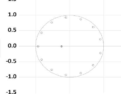
Figures 5, 6 show the Ljung – Box Q test and inverse roots of the ARIMA (13, 1, 1) model. Figure 5 present the results that the study fails to reject the null hypothesis. That is, most of the p-values of the test are greater than 0.05, which implies that the residuals for our time series model are independent. For a diagnostic of ARMA structure, the roots must lie right inside the unit circle. Otherwise, the model may be regarded as unstable and hence not suitable for forecasting. Since the corresponding inverse roots of the characteristic polynomial lie in the unit circle, then this paper can conclude that the chosen ARIMA (13, 1, 1) model is stable and indeed suitable for forecasting total public debt for South Africa.

Since the ARIMA model (13, 1, 1) is fairly describing the trend of total public debt and suggests better accuracy for further forecasting, then the equation (2) reflects the model specification as follows:

d ( dbtp ) _t = a + P 1 ^dbtp_t-1+ ...+ +^dbtp_t — ₁₃ + ^e t + (P 2 e_t —i + 8_t

In this paper, the equation (2) was used to determine the model that allows obtaining the forecast values of total public debt in South Africa.

Table 3. Analysis of best model selection

Model	Variables	Coefficients	t-statistics	AIC	Adjusted R-squared
ARIMA (1,1,1)	AR(1) MA(1) Sigmasq	0.657 -0.312 7.261	1.840** -0.708 7.746***	4.920	0.124
ARIMA (8,1,1)	AR(8) MA(1) Sigmasq	-0.166 0.355 7.484	-0.996 3.000*** 8.705***	4.953	0.097
ARIMA (13,1,1)	AR(13) MA(1) Sigmasq	-0.399 0.239 6.688	-1.837** 1.733** 6.662***	4.872	0.193***
ARIMA (1,1,12)	AR(12) MA(8) Sigmasq	-0.311 -0.119 8.048	-1.270 -0.793 10.193***	5.041	0.029
ARIMA (1,1,14)	AR(1) MA(14) Sigmasq	0.356 -0.201 7.087	3.838 -0.797 8.593	4.904	0.145

Figure 5. Ljung – Box Q statistics test for the model ARIMA (13, 1, 1)

Autocorrelation	Partial correlation		АС	PАС	Q-Stat	Prob
1                                     1	1                        1	1	0.03...	0.03...	0.058...
I 3i	1   ■	2	0.15...	0.15...	1.749...
1 ■	1 II	3	0.16...	0.16...	3.643...	0.05...
1 1 1	1 1 1	4	0.08...	0.05...	4.152...	0.12...
1 1 1	IC i	5	-0.0...	-0.1...	4.728...	0.19...
I Hi	1     ■ 1	6	0.18...	0.14...	7.041...	0.13...
1 11	1     ■ 1	7	0.10...	0.13...	7.893...	0.16...
HZ i	lEZ i	8	-0.1...	-0.1...	9.773...	0.13...
1 1 1	1 1 1	9	0.04...	-0.0...	9.920...	0.19...
1 11	1 II	10	0.13...	0.15...	11.31...	0.18...
1 1 1	1                  1	11	-0.0...	-0.0...	11.71...	0.22...
1 ■ 1	■ 1	12	-0.1...	-0.2...	12.99...	0.22...
1                     1 1	1 1 1	13	0.05...	-0.0...	13.26...	0.27...
!■ 1	1 1 1	14	-0.2...	-0.0...	16.73...	0.16...
1 1 1	1 11	15	-0.0...	0.10...	16.77...	0.20...
1 11	1 11	16	0.10...	0.09...	17.72...	0.21...
1 1 1	1                  1	17	0.04...	0.02...	17.93...	0.26...
!■ i	1 ■ 1	18	-0.1...	-0.1...	20.71...	0.18...
1 II	1     ■ 1	19	0.16...	0.13...	23.10...	0.14...
I E i	1 1 1	20	-0.0...	-0.0...	23.92...	0.15...
i 1 i	1 1 1	21	-0.1...	-0.0...	24.90...	0.16...
i 1 i	1      ] 1	22	0.11...	0.11...	26.12...	0.16...
1                        1	1 1 1	23	0.03...	0.03...	26.22...	0.19...
1 1 1	1 1 1	24	-0.0...	0.03...	26.57...	0.22...
1                                     1	I E i	25	-0.0...	-0.0...	26.58...	0.27...
1                                      1	i Ji	26	0.25...	0.15...	33.66...	0.09...
1 1 1	1                        1	27	-0.0...	0.01...	34.73...	0.09...
1 H1	1 и 1	28	0.14...	0.09...	37.03...	0.07...

Figure 6. Residuals AR roots for the model ARIMA (13, 1, 1)

D(DBT): inverse roots of AR/MA polynomial(s)

AR roots

• MA roots

-10  1

Forecasting results

Before we start to discuss the forecasted values, we should note that some of the forecasting evaluations were considered to gain the confidence in the forecast. Table 4 provides the evaluation criterions of forecasting ARIMA (13,1,1) model. The paper applied the most frequently used evaluation criteria’s such as Root Mean Squared Error (RMSE), Mean Absolute Error (MAE) and Mean Absolute Percent Error (MAPE). The paper explored the forecasting techniques which is dynamic forecasting to have a better sense of the results. In observing the results of the technique, it can be concluded that it provides better forecasting results.

Figure 7 demonstrates the trend of public debt (DBT) which is actual and forecasted (DBTF) using dynamic forecasting. The forecast for in-sample covers the period from 1960 to 2022, whereas out-of-sample is for one period ahead, which is 2023. It can be observed from the figure that the forecasted values mimic the data well of the actuals (Tab. 5) .

Table 4. Evaluation criteria of forecasting ARIMA (13,1,1)

Evaluation criteria	Dynamic forecasting
RMSE	11.44
MAE	8.01
MAPE	19.58

Table 5. Comparison of actual and forecasted public debt

Year	Actual values	Forecasted values
2021	68.8	71.53
2022	71.1	70.33
2023	–	68.66

Figure 7. Actual and forecasted values of public debt using ARIMA (13,1,1)

DBT – Actual dynamics of public debt

DBTF – Forecasted dynamics of public debt

Thus, the forecast for total public debt shows a decreasing trend from 2021 with 71.53%, 2022 with 70.33% and 2023 with 68.66%. The current study projections also suggest a possible decrease in the growth in public debt. It can be observed from the two forecasts that they do not drift too much from the actuals, especial for the year 2022.

Conclusion

This paper attempted to shed further light on modeling and forecasting public debt. The study proposed the implementation of univariate ARIMA model which allows us to model and forecast the values of government debt in the future. It should be remembered that such an achievement in forecasting the future public debt is critical for public debt management. The findings of this study demonstrate that ARIMA (13,1,1) model is the best fit and the model has passed all the necessary diagnostic tests. The study further forecasted the values of public debt using dynamic technique. The forecast shows that, there is an expected decrease in the growth of public debt in the future. It should be noted that such envisaged reduction of public debt has some economic aftereffects on South African economy. It is therefore recommended by this study that fiscal policy makers should adopt a strong fiscal reform to keep the public debt to a minimum. Therefore, such a decision my include raising tax revenue or curbing of public expenditure to stabilize public debt. Therefore, the practical contribution of this paper was the ability of the suggested model to mimic the actual values of public debts stock by using forecasting. The suggestion for further research is that future studies should consider regime shifts (episodes of low and high public debt overtime).