Modeling and Simulation of integrated steering and braking control for vehicle active safety system

Published Online March 2011 in MECS

As we all know that safety, economy and environmentalism are the three basic factors of the development of the modern vehicle. Kinds of active safety control system have made great progress, almost including each direction of the vehicle movement. New

This paper is supported by science and technology development project of Official of Beijing Municipal Education Committee (N0:KM200811232003)

security technology in the vehicle has been widely used and most modern vehicles are equipped with different forms of active safety systems such as Anti-lock Brakes System (ABS), Traction Control System (TCS), Electronic Stability Program (ESP) and other systems [1]. ESP improves the active safety of vehicle significantly. It is a new vehicle active safety control system based on the ABS and TCS, and has been equipped in many cars throughout the world. ESP is becoming an international hot spot of automobile active safety research. It not only integrates all the functions of traditional ABS and TCS, but can improve the stability of the vehicle under extreme driving situation. The function of ABS and TCS is to maximize the friction between the tire and the ground during braking and acceleration to improve the braking and acceleration performance while the ESP is used to control the vehicle yaw movement to prevent the oversteering for the improvement of the vehicle's cornering stability and security. ESP is not only the integrated of ABS and TCS, but also extends the capabilities of the ABS and TCS [2] [3].

There are many uses for the vehicle yaw dynamic control, in addition to active suspension system, engine torque distribution and braking intervention [4], many vehicles combine with active steering system, active braking system or integrated active steering system and active braking system to achieve automotive yaw stability control [5,6,7]. Driver assistance systems for vehicle dynamics primarily produce a compensating torque for yaw disturbances. Such control system can react faster and more accurately than the driver, when an unexpected deviation from the desired yaw rate occurs. The deviation is taken between the desired yaw rate (generated by a prefilter from the steering wheel input and the velocity) and the actual yaw rate (measured by a rate sensor). Also critical rollover conditions may be measured and feedback into a driver assistance system. With the continuous development of computer control technology, the integrated active chassis system becomes the mainstream gradually and also a research focus on the current vehicles stable control.

In this article, a research experiment platform based on the theory of vehicle dynamics, and the nature of the vehicles dynamics integration control combined software and hardware strategy which aims to study the integration of steering and braking control is designed. The integrated active steering and active braking control system is used to fulfill simulation, the Rapid Control Prototyping (RCP) and Hardware-in-loop (HIL) for the research of vehicle active safety control. For the requirement of the system, a seven-freedom vehicle model is constructed first and the approach of vehicle parameters estimation based on the Extended Kalman Filter is proposed. After an intensive study of nonlinear filter, such as Extended Kalman Filter, a 7-DOF vehicle model is built including vehicle dynamics model foundation for the estimation of tire forces. Combining the above 7-DOF model and making full use of the sensors—including sensors of acceleration, steering wheel angle, yaw rate and wheel speed, we can establish a new method to estimate tire force, which is most difficult to be measured directly, and the minimum mean square error estimation of longitudinal and lateral speed, longitude and lateral tire forces can be obtained respectively. The primary control methods and controller designment is carried out to prove the validation of the platform.

• II.    T HE S TRUCTURE A ND C OMPOSITION

The structure and composition of the experimental platform is shown in Fig. 1.

The platform includes a test vehicle which is equipped with the active systems of steer-by-wire and brake-by-wire and the Autobox, combined with the Matlab/simulink and MSCCarsim, is embedded too. CarSim simulates the dynamic behavior of racecars, passenger cars, light trucks, and utility vehicles. CarSim animates simulated tests and outputs over 800 calculated variables to plot and analyze, or export to other software such as the Matlab, Excel, and optimization tools. Use CarSim to design, develop, test and plan vehicle programs. CarSim allows users to make better decisions

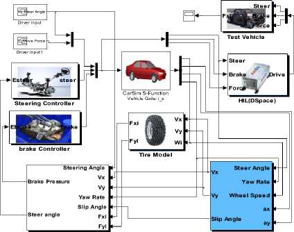
VDC Controller                                     EKF Estimator

Fig. 1. Construction of the integrated control system.

involving vehicle dynamics in less time. The software can be used to prove initial concepts, select components, and perform advanced analysis of existing vehicles.

The software, which includes tire model, parameter estimation module and the controller part is also provided in the platform.

• A.    Active steer-by-wire

The steer-by-wire system which is composed of an electronic control module, controller module and steering actuator module is equipped on the test vehicle (Fig. 2).

In steer-by-wire systems no direct transmission of power exists between steering wheel and the controlled tires in normal mode. Intermediate steps to real steer-by-wire are active steering systems. There, a conventional servo power steering is assisted by an electric motor to adjust the front wheels steering angle in proportion to the vehicles current speed. This affords a higher comfort in driving. Real steer-by-wire systems consist of several sensors, electro motors and controllers. Sensors, connected with the steering wheel, capture the input of the driver. To have a realistic driving feeling, a hand wheel actuator (HWA) gives the driver a haptic feedback of his input. Because there is no mechanical connection to the steering wheel, new innovative input forms, such as sticks, are possible to implement. A second electro motor, the front axle actuator (FAA), is placed at the steering rod and transforms the input signals in steering movements at the wheels. The operations of the actuators are coordinated by a central electronic control unit (CECU), which is connected by a real-time bus structure to the devices.

The main function of the electronic control module which consists of steering wheel angle poison and torque sensors and road feedback brushless DC (Direct Current) motor is to capture the steering wheel angle signal according to the vehicle drive’s intent and generate the appropriate expectations of the road feedback torque. The steering actuator which consists of brushless DC motor, position and speed feedback sensors and deceleration institutions, receives SBW controller output command and steers the front drive wheel through the steering torque motor deceleration. The primary function of the controller module is to accept the driver steering signal which is sent to active safety control system as a decision signal by the CAN bus and accept the final steering

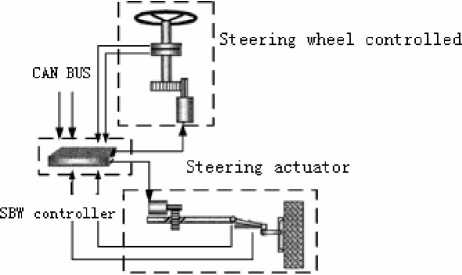
Fig.2. Construction of Steering by Wire command through the CAN bus to achieve the superimposition of the driver steering and the active steering angle. The controller is also responsible for the closed-loop control of torque feedback motor and steering motor to obtain the desired driver road feeling and control the front steering drive wheel accurately. From the structure and operation process of this system, it can be seen that the driver steering angle of steering wheel is only the reference signal of rotation angle and front wheel final steering angle is determined by active safety control system so as to achieve the active steering.

• B.    Active brake-by-wire

The brake-by-wire system in which the hydraulic power is used to create a more versatile braking system from MICO Incorporated, consists of an electronic pedal, a line drive, an electro-hydraulic modulating valve (EHV), a hydraulic power unit, the electronic control unit (ECU) and disc brakes (Fig. 3). ECU which communicates with the stability control ECU receives control instructions through the CAN bus. The pedal position from driver is only a desired reference signal and the final braking force is generated by the active safety controllers to achieve the active braking.

In evolution of vehicles the braking system is a basic module for driving safety. This system is subjected to a permanent development. Started with mechanic brakes, today hydraulic systems, assisted by inventions such as ABS, are the standard in cars. Nowadays development departments of all manufacturers are working on new brake-by-wire systems. First versions are still included in a lot of modern cars. The idea is that wires replace the hydraulic systems and commands are transmitted electronically through the wire [8, 9]. The built-in devices are electro-hydraulic brakes (EHB), where hydraulic and electronic components have been combined. A future solution will be the electro-mechanical brake (EMB). It totally forswears hydraulic components.

• C.    Configuration and designment of other hardware and software

AutoBox based on the Matlab/Simulink is the ideal environment for using your Dspace real-time system for in-vehicle control experiments such as ABS or chassis control development. AUTOBOX real-time system which

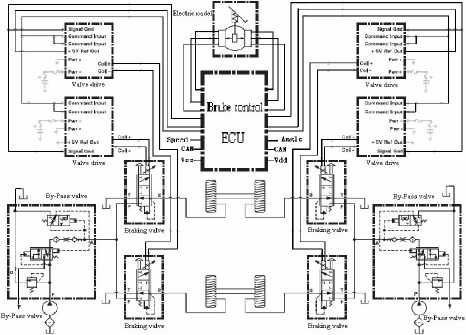
Fig. 3. Construction of Braking by Wire Hydraulic system can realize the RCP (Rapid Control Prototyping) and HIL (Hardware-in-loop) has a high-speed computing hardware system, including processors, I / O and etc, and its component is shown in Fig. 4. Also it was easy to realize the code automatically generated/download and testing/debugging. At the same time, the system for the RCP and HIL provides a tool of CDP (Control Development Package) which you can realize the entire process of the system modeling, analysis, off-line simulation, and until the real-time simulation. It is convenient that the developers just concentrate on the control scheme without the need for much time on the trivial chores, which can greatly reduce development cycle [10]. AutoBox is the ideal environment for using your dSPACE real-time system for in-vehicle control experiments such as test drives for the powertrain, ABS or chassis control development. You can install the AutoBox anywhere in a vehicle. AutoBox is a robust solution for mounting the processor and I/O boards in a car, aircraft or train. It provides space for Dspace hardware (up to 6 boards in the AutoBox, up to 13 boards in the Tandem-AutoBox). A Link Board for connection to the host is included.

This platform is used to implement software and hardware development of active safety systems and experimental work by AUTOBOX.

The special vehicle dynamics simulation software named MSCCarsim, which is developed through numerous research experiments and has higher accuracy, is used to overcome the difficulty and costly expense for achievement of the vehicle experiment data. The software combines traditional and modern multi-body vehicle dynamics modeling methods towards characteristic of parametric modeling for vehicle dynamics simulation software, including three-part graphic database of fullvehicle model, the direction and speed control and the external conditions (including the road information , drag, etc.) With CarSim's simple and easy to understand user interface, users can view full-vehicle model, simulation and results, so can use the simulation software quickly and accurately to provide a reference for engineering design.

The experiment and evaluation of the control system can be carried out through MSCCarsim under simulation environment and the needed data and results can be achieved conveniently. The CarSim math models cover the complete vehicle system and its inputs from the driver, ground, and aerodynamics. The models are extensible using built-in VehicleSim commands, Matlab/Simulink from the Mathworks, Labview from National Instruments, and custom programs written in Visual Basic, C language, MATLAB, and other languages. Use these options to add advanced controllers or extend the detail in subsystem or

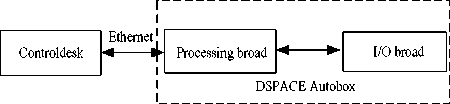
Fig. 4. The hardware system of Dspace Autobox component models such as tires, brakes, powertrain, etc. CarSim combines a complete vehicle math model with high computational speed. The software development team at Mechanical Simulation uses the VehicleSim Lisp symbolic multibody program to generate the equations for the vehicle math models. Besides providing correct nonlinear equations for fairly complicated models, the machine-generated equations are highly optimized to provide fast computation.

CarSim models typically run more than ten times faster than real time on a 3 GHz PC, so you always get results quickly. CarSim easily supports real-time (RT) testing with HIL systems using equipment from most RT suppliers. This speed also helps with software that requires many repetitions (optimization, design-of-experiments, etc.).

For the study of vehicle active safety control, the work of the designment and experiment can be done only after the vehicle model, force model between tire and ground, estimation for unmeasured state parameters have been carried out. The vehicle model used in simulations is briefly described. The fundamental control objectives are then explained for each system. Subsequently, the results of simulations are presented followed by conclusions. The following parts of this paper will focus on these assignments.

• III.    N ON-LINEAR S EVEN-FREEDOM V EHICLE M ODEL

• A. Seven-freedom vehicle model

The vehicle model used in this study was developed as a tool for testing of active chassis control systems at the development stage, as well as for hardware in the loop simulations. Vehicle dynamic model is the basis for control system design, a vehicle dynamic model with 7 DOF including the longitudinal speed, lateral speed, yaw rate and four wheels motion state is proposed in this paper and the list, pitch as well as vertical suspension dynamics and the roll motion are neglected for simplifying the research. The structure of the vehicle model is shown in Fig. 5.

The state equations of the vehicle are as follows:

Fxfl

vf vf

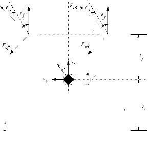
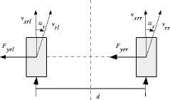
Fig. 5. 7-freedom vehicle model

•

x ( t ) = f ( x ( t ), u ( t ), t ) + w ( t ) =

V ,

•

V y

••

Yaw

to fl

•

^ fr

• to rl

• torr

—[( F , + F ,)cos 8 - ( F _n + F ,)sin 8 ] + F ,+ F + M * Yaw * V ] _M xfr xfl                 yfl yfr                 xrl xrr                      y

• 1                                                                                             •

M К F f ^{+ F} .f, ^{)sin 8 +} (F l ^{+ F} , ^)c os ⁸ ) ⁺ F yrl ⁺ F yrr ^- M * Yaw * V , ^] 2 j - K- F f ^{+ F} ,fr ^{)cos 8 - ( - F}y, ⁺ F yfr ^{)sin 8 ] +} 2^ (- F l ^{+ F}„ )

⁺ a К F f ⁺ F .fr ^{)sin 8 + (} F y, ⁺ F f ^{)cos 8 ] - b} (^F„ l ^{+ F}„ r )

^[ - R . F ., -K b T + T , ]

Iw

^[ - R . F ., - K f T + T ,r ]

Iw

— [- R F ,- KT ]

I w xrl brl b

w

Iw

Where ^Yaw is the yaw rate ( ^{rad / s} ), ^Vx and ^Vy are the longitudinal and lateral velocities respectively ( m / ⁵ ), ® ij

F is the wheel angular velocity (rad/s), ij is longitudinal and lateral tire forces (N ),R is the radius of the wheel (m ),Iz is the moment of inertia of the vehicle about its yaw axis (kg *m), a is the distance from the center of gravity to the front axle( m ),b is the distance from the center of gravity to the rear axle( m ),B1 and B2 are the front and the rear wheelbase respectively(m),8 is the front steering angle( rad ), Tb and Tf are the applied braking and drive torque respectively( Nm ).

The sideslip angles of each wheel are as follows:

a , = 8 - tan ^-

•

V y + a *Yaw

V, m0.5* B* Yaw a ri = tan

•

- V _y + b * Yaw V , m 0.5* B ₂* Yaw

,(, - front ; i = left , right )

, ( r - rear ; i = left , right )

The front and rear wheel center velocities are as follows:

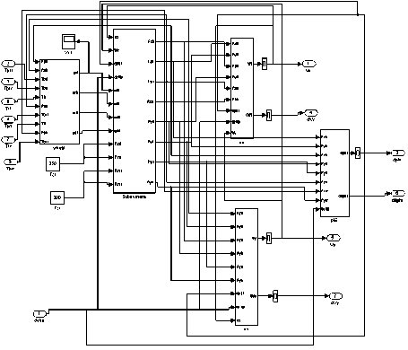
Fig. 6. simulink the vehicle model camber. Due to the fact that tires behave like nonlinear softening springs, transferring vertical load from one tire to another results in a net loss of lateral force. When a rolling tire is influenced with lateral force an apparent path is made with an angle relative to the wheel plane. This angle is referred to as the slip angle. Conversely, the slip angle can be used to determine the lateral force in conjunction with the aforementioned camber angle and the vertical load. The slip angle can be measured by specific sensors or back-calculated from a data acquisition system which measures vehicle lateral, longitudinal and vertical accelerations as well as vehicle yaw and pitch.

Pacejka Magic Formula model and the Dugoff tire model are two kinds of versatile algorithm which are used to model tire forces. Dugoff’s tire model (Dugoff, et. al., 1969) is an alternative to the elastic foundation analytical tire model developde by Fiala (1954) for lateral force generation and by Pacejka and Sharp (1991) for combined lateral-longitudinal force generation.

Dugoff’s model provides for calculation of forces under combined lateral and longitudinal tire force generation. It assumes a uniform vertical pressure distribution on the tire contact patch. This is a simplification compared to the more realistic parabolic pressure distribution assumed in Pacejka and Sharp (1991). However, the model offers one significant advantage-it allows for independents values of tire stiffness in the lateral and longitudinal directions. This is a major advantage, since the longitudinal stiffness in a tire could be quite different from the lateral stiffness.

Compared to the Magic Formula Tire Model (Pacejka and Bakker, 1993), Dugoff’s model has the advantage of being an analytically derived model developed from force balance calculation. Further, the lateral and longitudinal forces are directly related to the tire road friction coefficient in more transparent equations.

For Dugoff tire model of a single wheel [11], it is essential to know the friction coefficient to have a tire model. Therefore, the resultant front and rear friction coefficients are as follows:

CC C

Where ¹ , ² and ³ are the Burckhardt coefficients. In the case of the known characteristics of the road, road friction coefficient is only dependent on the lateral and vertical slip rate dependent. The influence of applying a small slip ratio X is obvious: it induces the rotation of the resultant force on the tire, thus changing the yaw moment on the car. The controller needs to resolve by what amount the slip at each tire needs to be changed by to generate the required change in the yaw moment, and to mitigate the effects of this change on the longitudinal and lateral motions. Thus, a more straight forward relation between the tire forces and the slip ratio would benefit the control design.

For the system studied in this paper, tire longitudinal force and lateral force are decided by the following equations:

(1)The front and rear longitudinal and lateral wheel slips are as follows:

S xij S yij

1 [® j * R w *^cos “ j ^- V j

V f L ^ * R w *^sin a

, ( i = front , rear ; j = left , right )

(2) The resultant front and rear wheel slips are as follows:

S_ra = S x- + S y- ,( i = 1,2,3,4)              ⁽⁸⁾

(3) Now, the front and rear longitudinal and lateral tire forces can be known accurately. The tire-force equations are as follows:

[ F

L yi

H resi = - Fzi

Sresi

On the Matlab/Simulink shown in Fig. 7.

C. Parameter estimation

H resi = [ C 1 (1 - e - C 2 " re ") - C 3 ^ resi ] 2 ,( i = 1,2,3,4)       (6)

Sxi

S yi

,( i = 1,2,3,4)

platform, the tire model is

Vehicle stability control is mainly based on the various parameters (e.g. lateral acceleration, yaw rate, etc.) of the motion that determine the appropriate control strategy and achieves the safe vehicle driving by the active control.

In general, most of the vehicle motion can be measured through a variety of vehicle sensors. Due to constrained by the current technical level, some important variables

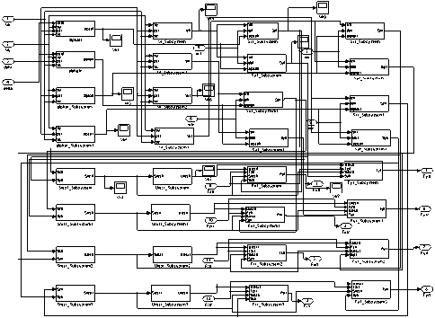
Fig. 7. simulink the tire model

need to use more expensive equipment to measure (such as speed, yaw rate), or even could not take direct measurements (such as the side slip angle), parameter estimation becomes a problem which must be solved on a vehicle stability control system designment. The most commonly used type of state estimator is nonlinear state estimation and Kalman filter.

The Kalman filter is a set of mathematical equations that provides an efficient recursive means to estimate the state of a process, in a way that minimizes the mean of the squared error. The filter is very powerful in several aspects: it supports estimations of past, present, and even future states, and it can do so even when the precise nature of the modeled system is unknown. The Kalman filter addresses the general problem of trying to estimate the state of a discrete-time controlled process that is governed by a linear stochastic difference equation. But what happens if the process to be estimated and (or) the measurement relationship to the process is non-linear? Some of the most interesting and successful applications of Kalman filtering have been such situations. A Kalman filter that linearizes about the current mean and covariance is referred to as an extended Kalman filter (EKF) [12, 13]. In something akin to a Taylor series, we can linearize the estimation around the current estimate using the partial derivatives of the process and measurement functions to compute estimates even in the face of non-linear relationships.

In the actual implementation of the filter, the measurement noise covariance R is usually measured prior to operation of the filter. Measuring the measurement error covariance R is generally practical because we need to be able to measure the process anyway (while operating the filter) so we should generally be able to take some off-line sample measurements in order to determine the variance of the measurement noise.

The determination of the process noise covariance ^Q is generally more difficult as we typically do not have the ability to directly observe the process we are estimating. Sometimes a relatively simple process model can produce acceptable results if one “injects” enough uncertainty into the process via the selection of ^Q . Certainly in this case one would hope that the process measurements are reliable.

In this paper, the extended Kalman filtering Filter (EKF) is used as the basic observer design tools [14, 15] for vehicle identification and state estimation because of its applicability, accuracy and simplicity. The identification and state estimation process of EKF is shown in fig. 8.

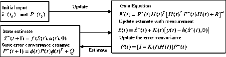
Fig. 8. Working process of EKF

For the system model, EKF process is carried out as following steps.

Step 1: The state equation and measurement equation of the vehicle

X ( t ) = f ( x ( t ), u ( t ), t ) + w ( t ) y ( t ) = h ( x ( t ), t ) + v ( t )

Where x(t) is the state variable, u(t) is the control variable, y(t) is the measurement output, w(t) is a white

Gaussian noise and its variance is Q , v(t) is the measurement noise and its covariance is R . w(t) and

^{v ( t )} are independent ， zero mean, Gaussian white noise which the probability distribution are as follows:

p(w) ~ N(0,Q)

p(v) ~ N(0,R)(12)

Q (t) = cov [ w (t), w (t )]

R (t) = cov [ v (t), v (t )]

According to seven degrees of freedom nonlinear vehicle model, we can get some variable as follows:

The state vector:

^{x (} t ) = [ ^Vx V y Yaw w f w r w rl w rr ] T ⁽¹⁵⁾

The measurement vector:

У ⁽ t ) = [ a x a y Yaw w l w r w l w r ] T     ⁽¹⁶⁾

The control input:

u ( t ) = [ 5 K_MT. KT K.,T. K T T„ К 1 ^{T    (17)}

bfl b brl b brl b brr b fl fr J

Where a and a are the vertical acceleration and xy lateral acceleration for the vehicle.

xxy av = V, + YOw * vr yyx

With the seven degrees of freedom vehicle model, the state equation is (1) and the observation equation is as follows:

y ( t ) = h ( x ( t ), t ) + V ( t ) =

a 1 x a y • Yaw		1, l< F f, + F f )cos 8 - ( F yf + F yf, )sin 5 ] + Fn M		+ F ,, ] + F,„ ]	(2Q)
		л 7[( F f Yaw	+ F f, ) sin 5 + ( F yfl + Fyf, )cos 5 ) + F,rt
to„	=	to,
to fr		to f,
to rl		to rl
to" _		to r		.1

Step 2: The linearization of the model

F ( t ) and H ( t ) are the Jacobian matrix which are derivative of nonlinear function f ( x ( t ), u ( t ), w ( t )) and h ( x ( t ), v ( t )), V t is the sampling time.

f f dx1      dxm

H ( t )

5 h ₁        5 h ₁

5 x "  " 5 xm

^{d h}m       ^д h m

m

Ф(t) = eF(‘),V‘ »I + F(t) *At (22)

The state equation of the vehicle substitutes into the (21), and you can get the state matrix and the measurement matrix as follows:

о Yaw v_y о о о о

F ( t ) =

- Yaw о - v_x о о о о

0   0   0  0 0 00

0   0   0  0 0 00

0   0   0  0 0 00

0   0   0  0 0 00

0   0   0  0 0 00

H ( t ) =

V & - Yaw

YOw &

- v_y о о о о v_x 0 0 0 0 1 0 0 0 0 0 1 0 0 0 0 0 1 0 0 0 0 0 1 0 0 0 0 0 1

Step 3: Choose an initial value for ^{x ( t 0)} and ^{P ( t 0)} and take the process shown as Fig.8 to achieve EKF filter recursive algorithm.

• IV.    P RIMARY E XPERIMENT R ESULTS

Parameter estimation by EKF, active steering control and active braking control are carried out in order to verify the feasibility of the system and model.

Parameter estimation input model for EKF is the (1) for first-order Taylor linearization by (21), and the observation equation by h (x (t), t) = [ ax, ay, r, tofi, tof,, to,i ,ш„ ] T + w (t)

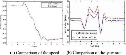
is obtained the equation (11) through first-order Taylor linear equation. In this paper, the initial speed is 95Km/s, road friction coefficient is 0.3. Actual vehicle parameters are obtained by MSCCarsim software and the estimated results of the speed and yaw rate compared with the actual values are shown in Fig. 9. It can be seen from the results that the estimated speed has a good match with the speed, but the estimates of the yaw rate has a certain degree of deviation with the real one. The reason may be the inappropriate selection for the value of Q and R .

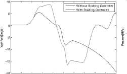
The active steering and active brake control which use sliding mode control [16] and optimal control respectively [17] for handling stability is carried out through the two-lane change movement of 120Km/h on a low friction road with the coefficient of 0.4. The control process is fulfilled based on (1) and MSCCarsim dynamics simulation system and the reference yaw rate is created by the linear two-freedom vehicle model. Comparisons of the active braking and active steering control results are shown in Fig. 10 and Fig. 11.

The comparison of the yaw rate between active braking control system and non-active braking system respectively is shown in Fig. 10 (a) and Fig. 10 (b) is the distribution of the braking force for a four-wheel active braking vehicle system. It can be seen from the figure that the vehicle using active braking can track the expected reference value better while the one without the active brake control systems falls off the expected vehicle trajectory after 2.5s and the vehicle is out of control.

The comparison of the steering angle with active steering control system and tradition steering system is shown in Fig. 11 (a) respectively. Fig. 11 (b) shows the

0.5

1.5

3.5

4.5

2    2.5    3

Time(s)

Fig. 9. Comparison of EKF parameters estimating result process of EKF

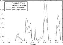
(a) Comparison of yaw rate (b) Distribution of braking force Fig. 10. Comparison of Active Braking Control Result

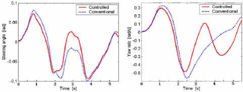
(a) Comparison of steering angle (b) Comparison of yaw rate Fig. 11. Comparison of Active Braking Control Result comparison of the yaw rate with active steering control system and non-active steering system respectively. The result from the figure shows that the vehicle using active steering can track the desired yaw rate accurately while the one without the active steering control system loses its stability and yaw rate deviate from the desired trajectory after 3s.

• V.    C ONCLUSION

An experimental platform combined with the software and hardware which aims to study the integration of steering and braking control is designed in order to develop the integrated active chassis system. The platform is used to fulfill active safety system simulation based on active steering and active braking control of vehicle, the RCP (Rapid Control Prototyping) and HIL (Hardware-in-loop). The seven-freedom vehicle model and Dugoff tire model are constructed first and the approach of vehicle parameters estimation based on the Extended Kalman Filter is proposed according to the requirement of the system. The primary control methods and controller design based on the active braking and active steering control is carried out to prove the validation of the platform for integrated control of braking and steering to provide theoretical and practical basis.