Modeling of Haze Image as Ill-Posed Inverse Problem & its Solution

Published Online December 2016 in MECS DOI: 10.5815/ijmecs.2016.12.07

Index    Terms —DCP,    Deconvolution,    Blind

Deconvolution, IP, Priori, Posteriori.

• I.    Introduction

  It is an area of applied mathematics, but traditional mathematics tries to avoid it where no solution, many solutions or missing conditions appear. In some cases equation produces matrices which are singular and as a result non invertible. In those situation multi –precision arithmetic is of no use. Therefore this can be concluded that inverse problem is a situation where answer is given, and the question has to be found out from a series of questions. Example is TV game Jeopardy. Forward or direct problem is the counterpart of inverse problem. Example of inverse problem is medical imaging, seismology, geoscience, remote sensing etc. They belong to deterministic problems. It has been found that majority of the real world problems are inverse in nature. Jacques Hadamard, French Mathematician 1923 proposed well posed problem in mathematics whose characteristics are 1. A solution always exists, 2. The solution is unique, 3. A small change in the initial condition produces a small change in the solution. The complement of this condition is ill-posed problem with charesteristis 1. Solution may not exist, 2. More than one solution may exist, 3. A small change in the initial condition may lead to large change in the solution. Thus inverse problem leads to ill-posed problem. Inverse problem was first identified by Victor Ambartsumian, Soviet Armenian theatrical astrophysicist .

Often IP does not follow well-posedness, and then IP becomes IP Ill-Posed Problem and becomes unstable. Visibility Improvement is also a class of inverse problem where best input or original image has to be found out from a series of probable input images. A well –posed problem may be ill-conditioned, i.e. a small error in the initial condition may produce significantly large error at the output /result. The trade-off between well-conditioned and ill-conditioned depends on the nature of the problem and its results[1,2].

Presence of haze degrades the outdoor images and videos to a great extent and thus has become a major problem for outdoor surveillance, driving, navigation in bad weather conditions. Poor visibility makes it difficult for the viewers to identify the object of interest. Dehazing has become an important research topic in many computer vision based applications such as video surveillance, remote sensing, object recognition, and tracking. Haze removal is a branch of Solving Inverse Problem. The focus of this paper is on the measure of effective haze removal algorithm with contrast control and sky masking from single image and video. Algorithm speed is an important parameter to measure complexity which is a linear function of image pixels. Therefore realtime application is can be correlated with algorithimic complexity, parameters like atmospheric veil inference, image restoration, tone mapping, smoothing are also the area of applications. The algorithm is equally equipped to handle both colour as well as gray image[3]. The nondeflected scene light reaching the camera together with the light reflected from different direction forms the airlight [4].Haze is caused due to scattering and absorption of light by tiny air particles known as aerosols in atmosphere before it reaches the camera [5]. This phenomenon fades the true color and contrast of the scene objects. Since haze is dependent on an unknown depth which cannot be measure accurately, dehazing an image completely becomes impossible but however improvement in visibility can be rendered by the various approaches of dehazing and visibility restoration. The various models that have been proposed till date includes, model proposed by Satherley and Oakley [7] and Tan and Oakley[11], assuming that the scene depths were known they formulated a physics-based technique to restore scene color and contrast without using predicted weather information. Narasimhan and Nayar[8] analyzed the color variation in scene objects under the effect of homogeneous haze based on a dichromatic atmospheric scattering model. They considered two images of the same scene taken at different time intervals. Scene contrast recovery using this model is somewhat ambiguous as the color of the haze and the scene points are almost same. Fattal [9] presented a method for estimating the transmission in hazy scenes taking into consideration that the medium transmission function and the surface shading are locally and statistically uncorrelated. The dark channel prior model by He et al[10]aimed at dehazing a single image based on the outdoor haze free image information, a common drawback of the above two methods   being their computational cost and time complexity.The dark channel prior model is effectively used in this work for real time application with reduced timing complexity[6,12]. After dehazing, the artifacts in the resulting image present mostly in the sky pixels were removed by masking the sky portion from the image, which resulted in improved output. The rest of the paper is organized as follows. In Section 2 the proposed method has been described. Section 3 presents the experimental results on both image and video, a comparison with a few previous methods is also contained. Finally applications have been discussed in section 4.

• A.    Elements of an Inverse Problem(IP)

Inverse Problem(IP) deals with mapping between object of interest ( called Parameters ) with the acquired information of the objects. The Mapping , also known as Forward Operator is detonated by Measurement Operator ‘M’ where ‘X’, normally a Banach or Hilbert space with parameters ‘x’, in the functional space of ‘M’ and acquired information ‘y’ in the data space ‘D’, also a Banach or Hilbert space.

y= M(x) for X ∈ X and у ∈ D     (1)

The above equation shows a relationship between parameters x and data y. It is clear from the the equation 1 that it is to find out parameters or points ‘ x’ in the functional space X i.e. X ∈ X from the knowledge of data y in the data set D i.e. У ∈ D . Therefore it is evident that MO ‘M’ provides optimum model from the existing data y which is considered to be reposed on parameters ‘x’. It is certain that a good modelling solely depends on the choice of search space ‘X’ and number of data ‘y’.

M ( Xi )= M ( x₂ )→ X1 =            , X₂ ∈ X (2)

If the equation 2 holds true then MO ‘M’ is called injective, where data y distinctively characterize the parameters x. It is an ideal case. In practical case MO ‘M’ is discrete in nature and data ‘y’ contains noise. But such MO ‘M’ is no longer injective.If ‘M’ is injective then it is very easy to construct inversion operator ‘M-1 ‘ to uniquely define the ‘x’ , the elements of ‘X’. The main attributes of MO is stability estimation. This estimation quantifies how errors in data influence measurement operator to reconstruct the points ‘x’ of ‘X’. ω is modulus of continuity.

_‖ Xi - X₂ ‖ X ≤ to (‖ M ( Xi )- M ( x₂ )‖ D )    (3)

Where (0 ∶ ℝ+→ ℝ+ is an increasing function with (0 (0) = 0 which quantify the modulus of continuity of the inversion operator M-1 . This inverse operator contributes the assessment of reconstruction error ‖ X1 - X2 ‖X based on data acquisition error on MO ‖M(%1)-M(■^2)‖p . A reconstruction is satisfactory if the noise in the data acquired does not amplified radically in       the       reconstruction               when to (X)=Cx , known as stability equation, wℎere C is constant and it is called that the Inverse Problem is well-posed. Otherwise if the noise is amplified extremely, so that reconstruction becomes unstable or too noisy. When <0 =|log |X||   a measurement error 10-10

produces a reconstruction error of 10-1 and the Inverse Problem is termed as ill-posed. Therefore Ill-posedness of IP is subjective. If   d(У1 , y2)=to(‖У1 - y2 ‖D), known as modulus of continuity equation, then the distance between two reconstruction x1 and x2 is confined between y1 and y2 which corresponds to a well-posed Inverse Problem. Therefore stability and continuity are subjective. У1 =   (%1 ) , y2 =   ( ■^2 ) dud. d (У1 , y2 )

are very important from the point of view error.

• B.    Noise, modelling, prior information

It has already been stated that MO is not sufficient condition to describe an IP. For practical or realistic modelling noise contributions have to be associated to the model, otherwise uninvited or unstable reconstruction will created. Therefore to stop this undesirable reconstruction prior information on the parameters have to be retrieved. Basic model of IP

• У =   ( x )                      (4)

Equation 4 is an ideal model. But real model is

• У =  ( x )+ n

и/ ℎ ere n is noise introduced in t ℎ e model (5)

The noise n has two folds. One is detector error or noise which is contributed by instruments and the other is modelling error which is coming from physical inherent system parameters of x with the data y. Noise is mathematically defined as the discrepancy between measurement operator M(x) and acquired data y.

n :=  - M ( x )                (6)

• 1.3 Prior Assumption: IP is classified by two parameters MO (Measurement Operator) and noise . Noise is required to be modeled owing to stability estimation associated with MO. Three conditioned have been aroused out of this problem, i) acquire more precise

data of lower size as at the time of stability estimation noise amplification may hamper reconstruction , ii) revise MO and attain altered data set if possible, iii) control the class where the unknown parameters are searched. There are various methods for prior assumption. 1. Penalization Theory. It is a deterministic theory. This is subdivided into a. Regularization, b. Sparsity Theory. 2. The Bayesian Framework, 3. Geometric constraint.

• C.    Penalization Theory

  • • • 1.3.1.1    Based on Regularization: Here у=  ( х )+

п is replaced by м∗у=(м∗м+ 8В ) х5          (7)

Where δ is a regularization parameter and B is a positive definite operator with м ^∗ м + дв an invertible operator of bounded inverse, M^* is an adjoint operator of M . In such a case IP becomes Linear system of equations.

• D.    Sparsity Constraints of Penalization

In this case У=  (х)+п replaced by х5 =        ‖У-М(х)‖Di +6‖х‖ ^2      (8)

Where δ is a small regularize parameter, D 1 is L² norm and X 2 is L¹ norm to promote sparsity. Such an IP becomes an optimization (minimization) solving problem. This equation eq (8) is more puzzling than equation (7).

• E.    Bayesian Frameworks

This model is more complex than those of previous models. Here a prior distribution π(x) assigns a probability (density) to all eligible candidates x before any data are acquired. This is also anticipated the likelihood function of the conditional distribution π(y/x), data y prior knowledge of parameter x. This is equivalent to knowing the distribution of the noise n. Bayes theorem expresses as

И ( X | У )= Си ( У | х ) К ( X )              (9)

Where C is normalization constant with probability density к(X|У ) and ∫ к п(X|У) йц (х)=1 withd/л (х) is a measure of integration on X. Two important Bayesian Methodologies are maximum likelihood, x = argmax π(х|У) = argmin - π(х|У)    (10)

This is MAP (Maximum a Posteriori Probability) Estimation and strongly resembles the equation 8 along with its computational cost and Equation 8 can be used as the MAP estimators of Bayesian Posteriori. Bayesian classical estimators are MAP( Maximum Posteriori), MSE (Mean Square Error), Maximum Likelihood(ML), Minimum Mean Square Error(MMSE),Maximum Mean Value of Error(MMVE). Hidden Markov model is an example of Bayesian model. Estimate-Maximize (EM) method. Estimation Theory (ET) is based on the selection of the optimum estimation of some parameters from a set of observed data. In case of signal to recover original signal from degraded signal with noise and distortion. Estimator receives the degraded signal and delivers an output which is as close as the original signal depending on the nature of the estimator and available data. Estimator may be a Dynamic Model (example, Linear Predictive (LP)) and/or a Probabilistic Model (PM) model (example, Gaussian model). Dynamic model predicts past and future values of the signals depending on its past course and present input. Whereas PM estimates the original signal depending on the given data fluctuations, SD, mean, covariance etc. [7].In statistics estimation is a newer data analytical model where probabilistic approximation of missing data is predicted. There are different estimators, like maximum likelihood, Bayes estimators, methods of moments, Cramer-Rao Model, minimum mean square error, minimum variance unbiased estimators, nonlinear system identification, best linear unbiased estimators, unbiased estimators, particle filter, Markov Monte Carlo , Kalman filter, wiener filter. If there are three equations and two unknown, it is known as over determined. If there are two equations and three unknown, that is known as Underdetermined.

• 1.3.3 Geometrical Constrain and Qualitative Methods: In this method available information cannot recovered wholly or partially the data set of x. This type of problem is computationally tractable than Bayesian Reconstruction [1].

• II.    Proposed Model

It has been observed that VI is a complex computational process. Any hazy image consists of haze as well as blur. Therefore both haze and blur removal algorithms have to be incorporated. In practice a lot of haze removal algorithms exist. DCP by He ET. AL , Fattal, Tarel, Tan name a few. In this paper DCP has been emphasised. Blur removal has been adapted by Regularization, Wiener, Inverse Filter, edge tapper, Lucy-Richardson, Blind Deconvolution. Haze removal is a time domain process, whereas blur removal is frequency domain process. Time domain operation always associated with colour shifting, so that image original colour may not be retrieved whereas frequency domain processing no such incident occurs.

• A. Improved DCP

  From the above discussion it is clear that VI (Visibility Improvement) is an IP. According to McCartney and H Kosmider in 1925[4] image visibility model is represented as

I(x) = J(x)t(x) + A(1 - t(x)) (1)

Where I(x) image viewed at a distance d. J(x) original scene radiance, t(x) transmission, A is the airlight scattered at the atmosphere.

t(x) =e-ра (2)

β is the scattering coefficient of the medium. The above equation indicates that the scene radiance is attenuated exponentially with the scene depth d. βd is known as optical thickness.

Jdark(x) = mince{r,g,b}(minyen(x)(Jc (y))) (3)

Jc represents the colour channel of J and Ω(x) is a patch around pixel x.The dark channel value of a haze free image Jdark generally tends to zero. This has been represented by the authors in [10] as:

Jdark(x) = minc(minyen(x)(Jc (y))) = 0 (4)

The colour of the most haze opaque pixels in I was taken as A.

• 1)    Atmospheric light estimation

It is carried out in the dark channel on 0.1% brightest pixels. It has already been stated that dark channel of an image estimates the amount of haze. Out of those pixels the highest intensity pixels are considered as atmospheric light. These pixels may not be the brightest in the whole image, but the method is robust and stable [4].

• 2)    Estimating Transmission

It is a heuristic model. To generate transmission map from a hazy image is an ill posed problem. To select an optimum transmission map is very difficult work. Haze free image along with good transmission map is the desired one .This can be evaluated from equation (1). Furthermore transmission ҄t for the transmission patch of size 15x15 with 7x7 padding is given by

t = 1 - min(c minyenco (^))      (5)

From eq (7) it is observed that in case of sky intensity value is one, same as that of atmospheric light A. This turns

min( min (^))) ^ 1

enw\ Ac / and

t ^ 0

Therefore this can be concluded that sky region has zero transmission. Eq (7) gracefully handles sky region without separating sky from rest of the image before processing. Now another interesting natural phenomena is being described that in sunny day little bit of haze prevails in the form of any free particle in the atmosphere. This is observed in very far object. Haze is a primary indication in the human perception of depth, called aerial perspective [7, 5]. Removing of haze completely from an image will make the image synthetic /unnatural and loose the sensation of depth. This pleasant phenomena is adapted artificially by introducing a parameter ω (0<ω<1) in the eq(7)

t =1-Ш min(c minyento (4?)) (6)

The value of ω is 0.95 in [10]. The value of ω can be tuned by using optimization.

• 3)    Recovery of Scene Radiance

It is an important term in association with poor visibility. The representation of scene radiance L(x, y, λ) enumerates the probability in visibility of noise, blur and colour difference in an image. A more complex depiction of scene radiance is L(x, y, z, θ, φ, λ) where transparency, depth of field and synthetic aperture are predicted. Therefore for efficient scene representation recovery of original scene radiance is essential.

/ (x) =          + A             (7)

( ( ),   )

Here a threshold value t 0 has been introduced, below which transmission is restricted. Typically the is assigned to 0.1.

• 4)    Contrast Controller

Most of the haze images suffer from degraded contrast of the scene objects. In this model contrast controller was applied after dehazing in order to shift the pixel values to fill the entire brightness range which results in high contrast .Here Michelson contrast has been used.

imax ^min ^max~ Imin

• 5)    Masking sky patches for removing artefacts and preserving the haze covered surrounding edges

It is observed that the resultant dehazed image obtained consist of a lot of artifacts present mostly in the sky patches, moreover the separation of edges of scene objects closer to the sky is not clear. Since sky is mostly blue the pixels for the sky were selected by picking values in the blue plane that are very high. The primary sky pixels were selected by keeping a threshold >200 and a mask was applied to each colour plane setting the mask pixels to a maximum value of 255.The resultant image obtained was visibly clearer and contained less artefacts. However the masking is only effective in daylight.

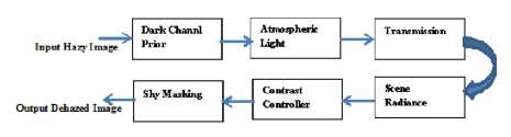
Fig.1. Block diagram of Proposed Haze removal model

• 6)    Results

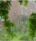
Here six available natural image set has been used. This has been shown in Table I with their entropies and size.. These images are different in quality wise, like indoor, outdoor, countryside, rainy, day, and night. But all of them have one similar quality, i.e., they are hazy.

Table 1. Original Image Set

Toys

Imag e

Entro py Size Imag e

Name Imag e

Entro py Size

Tree in rain

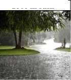
7.0414             7.8464

500x360,jpg Road

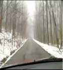
7.4136

532x352,jpg Foggy night

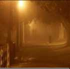
6.8289

House

7.1653

441x450,bmp

City

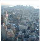
7.2058

804x446,png

1800x1200,jpg

576x768,jpg

The images of Table I have been passed through dark channel prior algorithm, then transmission estimation, after that radiance recovery stage, contrast controller and lastly through sky masking. The results of the dehazing technique are tabulated in Table II.

From the above table it is clear that after the above mechanism images are clearer than those of their original hazy counterparts

7) RGB Chanel Histograms

It is already known that work of He et al takes minimum 45 minutes to process a 50% reduced image with all necessary steps of the DCP [10].

Whereas it takes 7 seconds to run the proposed algorithm on a 50% reduced image. Although authors have used Matlab Image processing Apps whose results are given below. Demonstration of this app has been given only for the image canon.jpg. This app gives RGB channel intensity spectrogram for the channels. For a hazy image intensity of the pixels ranges 75 to 255. In case of images dehazed by He et. al., intensity varies between 0 to 175, 250-255.

Whereas our work of 50% reduced images take maximum 7 seconds. Now authors have used Matlab Image processing Apps whose results are given below. Here only one image named canon.jpg has been taken for explanation. In this apps each RGB channel intensity spectrogram has been shown. In the original hazy image intensity distribution occurs from 75 to 255 on and

average. In case of i) He et al 0 to 175 , 250-255, ii) guided filter also25-255 and iii) our method 0-150. This observation validates that our method discards haze well as high intensity values are less in our method. At the same time by visual experience our method explores extreme far road clear vision which is not clear in case of other two methods. Therefore it has been established by qualitative as well as quantitative analysis that our method is superior to earlier two methods.

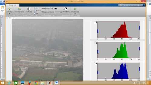
Fig.2. Hazy canon image and its individual RGB channel intensity distribution

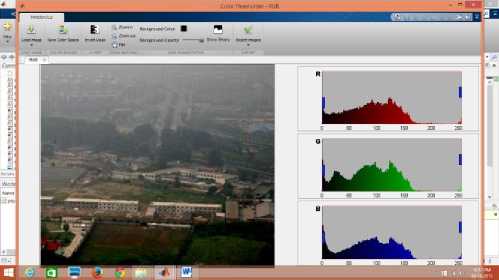
Fig.3. Haze free canon image and its individual RGB intensity distribution using He et al algorithm with soft matting

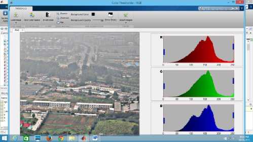
Fig.4. Hazefree canon image and its individual RGB intensity distribution using guided filter

Table 2. Qualitative Analysis of the Images used in Table I using proposed model

Sl no

Dark Channel Prior

Z i       Image

After Masking

Transmission

Radiance

Radiance Clear

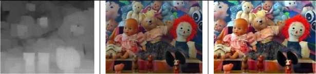
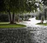
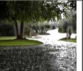
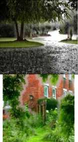
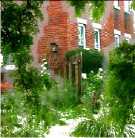
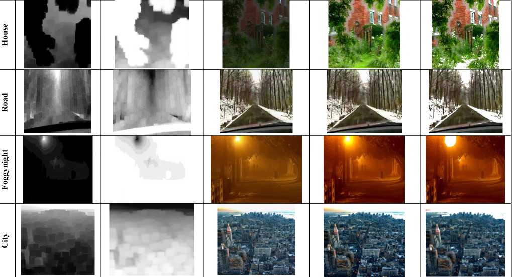
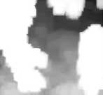
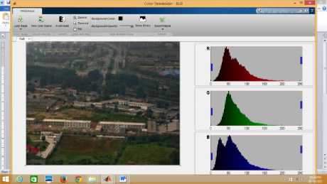
Fig.5. Hazefree canon image and its individual RGB intensity distribution using our method without soft matting

B. Blur Removal

Numerous improved visibility Improvement methods have been developed which give more efficient real time with less computational complexity[5][6]. Still a stint of blur prevails in the recovered image. This can be eliminated by Deconvolution [13].

1) Deconvolution

In signal processing most of the time original signal loses its originality due to the cumulative effect of noise and other factors from the source to destination. Main objective of signal processing is to retrieve back its original condition. But it is difficult to achieve as in time domain signal frequency components are mixed. This is easier to implement as in frequency domain all frequency components can be identified precisely and individually. In DE convolution frequency domain operation can be performed on the signals. DE convolution is a process by which image contrast and resolution improve[8]. This employs Fast Fourier Transform (FFT). At the time of transformation signal loses some information in the irregular region where pixel intensity changes abruptly. In image restoration deconvolution is one of the most useful methods of image blur restoration. Blur can be removed by Deconvolution with Regularize Filter, Wiener Filter, Edge Tapper, and Blind Deconvolution.

Table 3.Qualitative Analysis

Sl. No.		Original Degraded Image	Improved Output of Algorithm 1 7    '	Improved Output of Algorithm 2	Improved Output of Algorithm 3	Improved Output of Algorithm 4	Improved Output of Algorithm 5	Improved Output of Algorithm 6
		* *#4 T^H		7.4	, 8	A    V I         ‘	;'.p. 9
Opinion1	6.5		7			7.8		7.7
Opinion2	6		7.1	7.5	8.2	7.9	9	7.9
Opinion3	6.2		7	7	8	7	8	7
Opinion4	6		6.8	7.1	7.7	7.6	7.9	7.8
Opinion5	5		6.5	7	7.2	7.4	7.5	7.6
Average		5.94	6.88 ;'■•/■ ■	7.2 НЯК7--	7.82	7.54	8.28	7.6
Opinion1	8		7.5	7	7.1	6.8	7.1	6
Opinion2	7		8	7.5	7.3	6.5	7.5	6.7
Opinion3	6.4		7.5	7.8	8	6	7.8	6
Opinion4	6		7.1	7.3	7.9	6.9	7.5	7
Opinion5	5.9		7	7.2	7.5	6.7	7.2	7
Average	6.66		7.42	7.36	7.56	6.58	7.42	6.54
			1 1		$1	4	J.	15 ’
Opinion1	6.5		7.1	7.2	8	7.4	7.5	7.6
Opinion2	6		7	7.1	7.5	7.3	7.6	7.7
Opinion3	7		7.4	7	7.3	7	7.6	7.8
Opinion4	6		7.1	7.3	7.2	7.6	7.8	8
Opinion5	6.2		7.3	7.2	7.4	7.5	7.7	7.9
Average	6.34		7.18	7.16	7.48	7.36	7.64	7.8
		___ ■ - —	m	8!
Opinion1	6.4		8	7.9	7.5	7.7	7.9	8
Opinion2	7		7.9	8	7.3	7.9	8	7.7
Opinion3	7.5		7.7	8	7.6	7.8	8	7.9
Opinion4	6.8		7.5	7.8	7.9	7	7.8	9
Opinion5	6.7		7.4	7.7	7.6	7.7	7.6	8.1
Average	6.88 ■L W		1    4 1	7.88		7.62	7.86	8.14
Opinion1	7		7.1	7.8	7.6	7.5	7.2	7
Opinion2	7.1		7.7	8	7.9	7.7	7.6	7.1
Opinion3	7		7.5	7.8	7.7	7.3	7.9	7.4
Opinion4	6.8		7	7.3	7	7.1	8.1	7.6
Opinion5	6.7		7.1	7.2	7.5	7.0	7.5	7.5

Table 4.Quantitative Analysis

Sl. No.	Original Image	Dehazed DCP Output[6,12]	DCP  Deconvolved Regularized Output	DCP Deconvolved Winer Output		DCP  Deconvolved Edge      Tapper Output	DCP       with Deconvoled Lucy-Richardson Output	DCP with Blind Deconvolved Output
Image 1	MB,	Г • —, x ^	Ai^ 1 '         t		1 ? 1 > Ar^ ■ '^ J fl	<* r . Rv; '^	/Ъ^ r$
Entropy	7.0427	6.6991	6.7000	6.7000		6.7004	6.6916	6.6923
PSNR	-	6.0386	6.0411	6.0412		6.0388	6.0313	6.0325
SSIM	-	0.3259	0.3209	0.3209		0.3259	0.3193	0.3205
Visible Edge	16313	62767	66963	66963		66963	66963	66963
CNR	48.2731	63.9694	60.5380	60.5380		60.5380	60.5380	60.5380
Entropy	7.8464	7.5696	7.6228	7.6228		7.5657	7.6265	7.6221
PSNR	-	16.8702	16.4050	16.4010		16.8678	16.3766	16.4640
SSIM	-	0.8484	0.7851	0.7846		0.8481	0.7839	0.7940
Visible Edge	19016	17809	16758	16758		16758	16758	16758
CNR	80.6731	100.5406	103.3261	103.3261		103.3261	103.3261	103.3261
Image 3	VI 1 Я1 ^		1		1.
Entropy	7.1653	6.0937	6.2359	6.2370		6.0887	6.2365	6.2232
PSNR	-	10.6565	10.6697	10.6697		10.6537	10.6675	10.6679
SSIM	-	0.5361	0.5431	0.5430		0.5355	0.5431	0.5433
Visible Edge	19499	24605	24722	24722		24722	24722	24722
CNR	96.9151	42.8313	47.8643	47.8643		47.8643	47.8643	47.8643
Image 4					^^^^ ^^^j^			:               '/■■■'
Entropy	7.4136	7.6156	7.6731	7.6729		7.6135	7.6762	7.6750
PSNR	-	12.7618	12.5301	12.5290		12.7653	12.5203	12.5393
SSIM	-	0.7359	0.6737	0.6733		0.7349	0.6729	0.6773
Visible Edge	19600	23235	22959	22959		22959	22959	22959
CNR	94.0200	100.3251	101.6580	101.6580		101.6580	101.6580	101.6580
Image 5			T		*
Entropy	6.8289	6.4881	6.4966	6.4967		6.4872	6.4966	6.4964
PSNR	-	24.6196	24.6068	24.6066		24.6099	24.5999	24.6005

SSIM	-	0.9773	0.9770	0.9770	0.9773	0.9770	0.9770
Visible Edge	36418	41546	46403	46403	46403	46403	46403
CNR	14.4681	15.2308	15.0801	15.0801	15.0801	15.0801	15.0801
Image 6		■■■Ei'S'		, I. .
Entropy	7.2040	6.9515	7.1698	7.1707	6.9690	7.1686	7.1589
PSNR	-	14.6707	14.4202	14.4185	14.6680	14.4132	14.4323
SSIM	-	0.8252	0.7604	0.7600	0.8192	0.7599	0.7641
Visible Edge	41779	43623	40609	40609	40609	40609	40609
CNR	76.7152	86.1990	103.0721	103.0721	103.0721	103.0721	103.0721

7.28

Average

6.92

7.62

7.54

7.32

7.66

7.32

Opinion2

7.8

7.8

7.6

8.1

7.5

7.4

7.3

7.7

7.2

7.9

Opinion1    6.9                7.3

Opinion3

7.1

7.4

7.6

7.9

7.9

7.5

Opinion4

7.8

7.4

7.6

7.9

7.6

7.5

Opinion5

7.2

7.7

7.8

7.9

7.7

7.5

7.4

Average

7.04

7.6

7.54

7.7

7.84

7.48

7.78

• III.    Experimental Results

In table III and IV six different types of degraded image have been evaluated with respect to subject and object. Subjective evaluation has been carried out with the help of human opinion of five different persons and each of them has given in same position of different images, i.e., if human one has given his judgment for the opinion 1 in first image, then that person has given in opinion 1 for rest of the images. Average opinion has been evaluated for each image. This is clear that all algorithms are remarkable to remove degradation except rainy image of Image 2. Image 2 category is proven to be worsened. Parameters used for objective evaluation are entropy, PSNR, SSIM, CNR, and visible edges. Objective evaluation shows better result with respect to original image for all images, except Image2. Here number of visible edges degrades, SSIM increases, PSNRs are high with respect to other results, and entropies have been decreased. Whereas CNR in category 6 has been improved.

• IV.    Applications

This technique can be applied in surveillance, military, night vision, security, under water vision, remote sensing, driving aid, navigation, air traffic control, astronomy, old image restoration, and aerial image correction.

• V.    Conclusions

In this work the technique used is a novel method for dehazing in the scene that has been done on both video as well as image frame by frame. We have completely masked sky patches, which has not only resulted in an enhanced image but has also reduced artifacts along the surrounding edges. The final output is comparable with the existing techniques and quite suitable for real time video processing as the time taken for processing each frame is very less. The novel method has been applied on six images which gives satisfactory as well as efficient result in eight quantitative parameters. According to human opinion which is the last and final option in case of image, qualitative performance has also been found to be satisfactory. However in case of dense fog on applying the dark channel prior model the resultant image turned dark. Thus the future work of this model will stress on improving visibility in case of denser fog. This method is very simple and fast compared to He Et. Al. work. He Et. Al. work takes 45 minutes to complete a 50% reduced single image. Whereas our work takes only maximum20 seconds to complete the same image. The above mentioned methods can be implemented on any type degraded image and better results are produced, even motion blur can be removed. This has also been noticed that degradation in visibility of images has a tendency towards blurring.. For this reason deblurring methods have been integrated for better visibility improvement. After IDCP steps , deblurring algorithms like regularize filter, wiener filter, edge tapper, Lucy-Richardson , and Blind deconvoluton methods have been applied and the output have been observed sequentially. In all of the cases improvements have been observed which have been validated thorough qualitative and quantitative analyses. It has also been reported that all types of degradation are improved through these algorithms except in rainy scene. In future rainy image will be taken care for evaluation for algorithmic improvement.

Acknowledgement

In this paper authors have used Matlab Version R2014a for the experimental result. It is working under windows8 environment. Matlab Apps for RGB channel histogram has been used to show dark channel importance by visual representation.