Modeling of the organic Rankine cycle based on the theory of energy chains

Бюллетень науки и практики / Bulletin of Science and Practice

UDC 621.372.2                                     

The study of hydraulics and heat transfer processes is crucial for understanding and optimizing various engineering systems. Mathematical modeling, particularly using differential equations, has been widely used to address this challenge. However, the complexity of hydraulic and heat transfer systems often requires a systematic approach to model development and analysis.

In recent years, the application of energy circuit theory to describe hydraulic and heat transfer processes has gained attention. Despite the growing interest in these methods, there is still a need for a comprehensive study that combines the energy circuit approach with differential equations and black-box modeling to describe hydraulic and heat transfer processes.

The novelty of this work lies in the integration of energy circuit theory, differential equations, and black-box modeling to create a unified framework for describing hydraulic and heat transfer processes. The proposed methodology involves building an energy circuit, compiling equations, setting input and output through the black box, calculating equations using the black box, writing equations for the image, compiling the complex resistance equation, distinguishing coefficients, writing the frequency function for the energy circuit, and distinguishing the real and imaginary parts of the complex resistance to calculate the amplitude-frequency and phase-frequency characteristics.

Material and methods of research

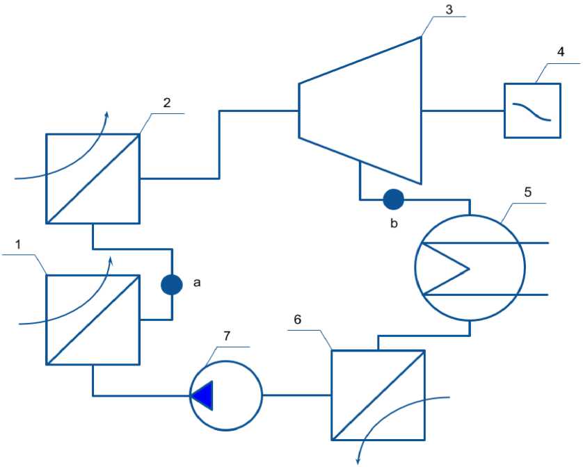
Figure 1. Experimental device for organic Rankine cycle

Table 1

SYMBOLS IN FIGURE 1

Position	Name
1	Evaporator
2	Superheater
3	Turbine
4	Generator
5	Condencer
6	Cooler
7	Pump

The principle of operation of the experimental setup

Figure 2 shows an experimental installation of a waste heat exchanger with a phase change.

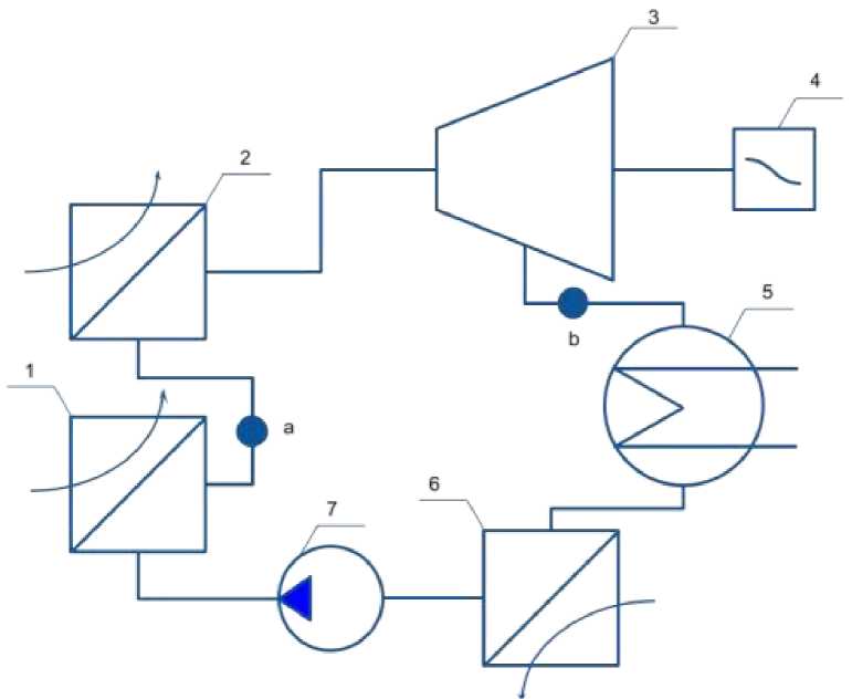
Figure 2. Experimental device for organic Rankine cycle: 1 – evaporator; 2 – superheater 3 – turbine; 4 – generator; 5 – condencer; 6 – cooler; 7 – pump

The working steam generated in the evaporator 1 reaches the turbine 3 through the superheater 2 for improving energy potential. After producing a work in the generator 4, low-potential gas make a phase change to the fluid in the condencer 5. After decreasing of temperature in the cooler 6, working fluid reaches to the pump 7. The heat transfer principle is shown in Figure 5.

In the course of the study, for a better understanding of the scheme, it was decided to study 2 characteristics of hydraulic and thermal, in order to better understand the nature of the forces arising and to more accurately determine the required parameters on the obtained model.

The first is hydraulic, which takes into account elastic properties of a spring with pliability 11 (pliability is the inverse of elasticity), inertial properties of a liquid by mass m1, pressure losses in the pipeline by means of active resistance r1. The third part is the network pump, and elastic properties of the spring with pliability 11 (pliability is the value of the inverse elasticity) cylinder walls by active resistance.

In the first power circuit the hydraulic characteristics at the moment of closing of the shock valve is considered. This circuit contains 2 elements.

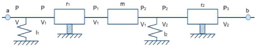
Figure 3. Hydraulic circuit

The circuit link equations:

Г p = r₁V₁² + m 1 V 1 + r₂V ? + P₃ {    V = l i P + I 2 P 2 + V 2

Black box:

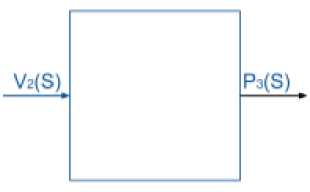
Figure 4. Black box for hydraulic energy circuit

Equations for P₃,P₂,P 1 :

P3 = P30 + P3

P2 = r2V22 + P3

P1 = mV1 + P2

Equations for V₂,V 1 :

V2 = V20 + V2

Vi = I2P2 + V20 + V2

Equation for P2:

P2 = r2V22 + P3 = r2V22o + 2^20^2 + P30 + P3

Equation for P2:

P2 = 2^20^2 + P3

Equation for V 1 :

Vi = 2l2r2V2oV2 + I2P3 + V20 + V2

Equation for V 1

⁵ 1 = ² ^ 2 ^Г 2 ^ 20 ^ 2 + ^/ 2 ^P 3 + ^К 2

Equation for K 2 :

К20 + (^'г^О5 + /2P3 + 52)] ~ 520 + 2^2o(2^2r2^20^2 + /2P3 +^

Equation for K22:

^22 = 520 + 2К2 0Ё2 + 1'2

Equation for P:

P = 71(^220 + 4^ЛГ2!>2 + 2^2 0^2Рз + 2^2 0^) + т^^оК + /2P3 + 5)

+ Z^V 2^ 20 ^ 2 + 5 2 ) + P 30 + Р з

= т^з + 27 1 / 2^3 + P 3 + P 30 + 2™^^ + М^лМ + mJ

⁺ I^ 2 ^(4r 2 ⁵ 2 0 ^{+ 2} ' 1 ⁵ 2 0 ^{) + 2} ' 2 ⁵ 2 0 ⁺ ' 1 ⁵ 220

Equation for images:

(a 1 s² + a₂s + a₃)V₂(s) = -(b 1 s² + b₂s 1 + b₃)P₃(s)                          (14)

Coefficients:

a 1 = m 1 /₂ ^a 2 = ² ' 1 ^/ 2 ⁵ 20 а з = 1 ^b 1 = Zm^' z^O b 2 = 4/ 2 ' 1 7 2 К₂²_о + m 1 ^b 3 = ^4r 2 ⁵ 20 ^{+ 2} ' 1 ⁵ 20

Complex circuit resistance Z (s):

( , _ P3(s) _ a1s2 + a2s + аз

^(s) = y 2 (s) = —b 1 s² — b 2 s —Ь з

Frequency function of the circuit:

s ^ jQJ2 = -1

Frequency function of the circuit:

—a 1 b 1 fi⁴ + a₁b₃fi² — a₁b₂jfi³ + a₂b₁jfi³ — a₂b₃jfi — a₂b₂fi²

+a3b1fi2 — a3b3 + a3b2jfi

=                        (b 1 fi² — Ь_з)² + b₂²fi²

Г—a 1 b 1 fi⁴ + (a₂b 1 — a₁b₂)jfi³ + (a₁b₃ — a₂b₂ + a₃Ь₁)fi²l

₌ L________________ +(a з b 2 — a 2 b з ⁾jfi — a з Ь з ________________ J

(b 1 fi² — Ь_з)² + b₂²fi²

The real part of the frequency function:

—a 1 b 1 fi⁴ + (a 1 b з — a 2 b 2 + a з Ь 1 ⁾ fi² — a з Ь з                            ⁽¹⁹⁾

^e(jfi) =------------------------------5--------------

(b 1 fi² — Ь_з)² + b₂²fi²

Imaginary part of the frequency function:

.          ^(а 2 ^ 1 - ^а 1 ^ 2 )^³ + ^(а 3 ^ 2 - ^a 2 ^ 3 ^)a .

Im(]a) =] (Ь1П2 - ь3)2 + Ь22П2

Amplitude-frequency response (frequency response) of the circuit:

А(]П) = ^Re(jO)2 + Im(jO)2

Phase frequency response (FFC) of the circuit:

Im(jO)

^(ia) = -arctBR^

Figure 5 shows the part of the installation where heat transfer takes place.

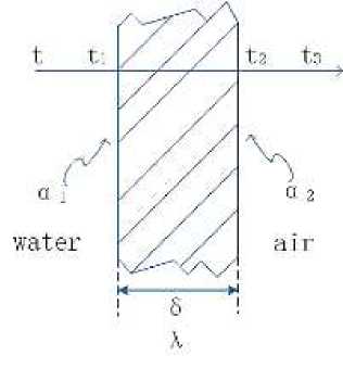
Figure 5. Part of the heat transfer plant: t - the temperature of hot water; t₁ ， t₂ - wall temperature; t₃ -the temperature of the air; α 1 - convective heat transfer coefficient of water and left wall; α 2 - convective heat transfer coefficient of air and right wall; δ - the thickness of the wall surface; λ - Thermal conductivity of the wall

When the hot water flows, the convective heat transfer coefficient between the water and the left wall is h 1 , and the temperature of t is greater than t 1 , so the wall absorbs the heat brough by the hot water, and the wall temperature rises. When the temperature rises to t 1 , the surface temperature of the left wall is stable. The thickness of the wall is λ, and the heat is transmitted from the left wall to the right wall by means of heat conduction. When the temperature rises to t 2 , the surface temperature of the right wall reaches a stable state. The right wall carries out convective heat transfer with the air, and the convective heat transfer coefficient is h 2 . Through convective heat transfer, heat is transferred to the air until the air temperature t 3 reaches a stable state.

Calculate the convective heat transfer thermal resistance r 1 :

r1 = a1F

Calculate the convective heat transfer thermal resistancer2:

^r 2

Calculate the convective heat transfer thermal resistance r3:

^r 3 =^ ^ 2 ^

Total thermal conductivity k.

1      _         1                                          (26)

r 1 +r₂ + г₃     1     8     1

a 1 F ⁺ AF + a₂F

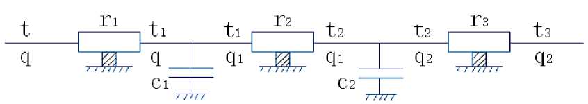
Figure 6. Heat transfer energy circuit

The circuit link equations:

1 1 = ГД + ЪЯ 1 + Г з Ц 2 + 1 з

I q = C i t i + C 2 t 2 + q 2

The input and output of the energy chain for thermal calculation are presented in the form of a “black” box.

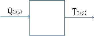
Figure 7. Black box for heat transfer

Equations for t₃,t₂,t₂,t 1 ,q₂:

^3 = t30 + t3

t2 =r3q2+ t3

t2 = t2 = r3q2 + t3

ti=r2qi + t2

q2 = q20 + q2

Equations on q 1 from the 1st link:

qi = C2t2 +q2 = С2(т3к + £3) + q20 +q2= C2r3q2 + C2t3 + q20 + q2

Equations on t2 from the 1st link:

t2 = r3q2 + £3 = r3q20 + r3q2 + £30 + ^3(34)

The equation on t 1 :

I^i = r2qi + ^2 — r2(c2r3q2 + ^^ + q20 + Я2) + (ГзЯ20 + Г3Я2 + t30 + ^3)

= С2Г2Г3Я2 + £2^3 + Г2Я20 + Г2Я2 + Г3Я20 + ^3^2 + t30

^{— c} 2 ^r 2 ^r 3 ^q 2 + ^(r 2 + ^r 3 ^)q 2 + ^(r 2 + ^Г3^)я20 + ^С2^Г2 * 3 + ^ 3 + ^t 30

The equation on t_i :

ti — c2r2r3q2 + (r2 + ^2 + c2r2t2 + t3

The equation on я :

Я — Citi + c2t2 + Я2(37)

— C i [c₂r₂r3q₂ + (r 2 + Г 3 )Я 2 + C₂r₂t₂ + t₃] + С 2 (г 3 Я 2 + £ 3 )

⁺ ( ^Я 20 ^{+ q} 2 )

^{— с}1^с2^г2^г3^Я ₂ ^{+ (c} i ^r 2 ^{+ c} i ^r 3 ^{+ C} 2 ^r 3 ^)q 2 ^{+ Я} 2 ^{+ Я} 20 ^{+ C} i ^C 2 ^r 2 t 2

+ (C i + C 2 )t₃

The equation on t:

1 — Г 1 Я + Г 2 Я 1 + Г 3 Я 2 + t 3                                                                    (38)

— r i [c i C 2 r 2 r3q₂ + ⁽ C i r 2 + C i r 3 + C 2 r^ 2 + Я 2 + Я 20 + C i C 2 r 2t2

+ (C i + C 2 )t₃] + ^2^2 + C 2 t 3 + Я 20 + Я 2 ) + Ъ⁽Я 20 + Я 2 ) + { 30 + * 3

— [с 1 С 2 Г 1 Г₂Г 3^ ₂ + ⁽ C i r i r₂ + C i^3 + C₂r i r3)q 2 + r i q 2 + Т 1 Я 20 + C i C 2 r i r₂t₂

^{+ (c} i ^r i ^{+ с}2^Г1^)£3^ ^{+ (c} 2 ^r 2 ^r 3 ^q 2 ^{+ С}2^Г2 * 3 ^{+ r} 2 ^q 20 ^{+ r} 2^Cl2 ^{) + (r} 3 ^q 20 ^{+ r} 3⁽ 1 2 ⁾

^{+ t} 30 + ^

— С 1 С 2 Г 1 Г 2 Г 3~ Я₂ + ⁽ C i r i r 2 + C i r i r 3 + С 2Г1Г3 + С 2 Г 2 Г 3^ Я 2 + (r i + r 2 + ^2

+ (r i + r 2 + ^20 + C i C 2 r i r 2 t 2 + (С^ + С 2 П + C 2 r 2^3 + t 3 + t 30

— biq₂ + Ь 2 Я 2 + Ь₃Я 2 + Ь₄Я 20 + aih + a 2 t₃ + chh + a^

Equation for images:

(d i S² + ( 2 $ + a^T^s) — - ⁽ b i S² + b 2 S + b3^Q 2 ⁽ s' ⁾                     (39)

Coefficients:

d i — C i C 2 r i r 2                                                (40)

( 2 — C i r i + C 2 r i + C 2 r 2

^а 3 ^{— 1}

b i — C i C 2 r i r 2 r 3

b 2 — C i r i r 2 + C i r i r 3 + C 2 r i r 3 + C 2 r 2 r 3

b 3 —r i + r 2 + r 3

Complex resistanceZ(s):

,   T 3 ⁽ s)   -b i S²-b 2 S-b 3                                (41)

Z (s) — тт-гт —---?----------- Q 2 (s)    a_is² + a₂s + a₃

Frequency functions of the circuit:

s ^ j^,j² — -1                                         (42)

Frequency function of the circuit:

= T3(s) = —bis2 — b2s — b3 = Ь1°2 — Ь2}° — ^3

Q2(s) p1s2 + p2s + а3 —а1О2 + а2]О + а3 (biO2 — Ь2]О — b3)[(—а^О + а3) — а2]О]

[(—а 1 О² + а₃) + а₂]О][(—а 1 О² + а₃) — а₂Щ]

(

—a₁b₁O⁴ + a₃b₁Q² — а₂b₁jO³ + я₁Ь₂]О³ — +a₁b₃O² — a₃b₃ + a₂b₃jO

аз^Щ — а 2 Ь 2 ^²^

——а1Ь1^4 + (а1Ь2

(—а 1 О² + а₃)² + а 2 О²

— a₂b₁)jQ³ + (u₃b 1 — a₂b₂ + a₁b₃)O² +

(P^ —aзb2')}O —aзbз

]

(—а 1 О² + а₃)² + а^²

We derive the real part of the complex resistance:

„ (    _  ^а1^1^^{4 + (р}3^Ь1  ^^ ^{+ а} 1 ^ з )^^{2   Р}3^Ь3

^¹⁾ =          (—а 1 О² + а₃)² + а^О²

We derive the imaginary part of the complex resistance:

,   .    (а1Ь2

Im(j^) =----

— a 2 b 1 )a³ + (a 2 b з

—

азЬ2№

(—а 1 О² + а₃)² + а₂О²

We obtain the amplitude-frequency function of the energy circuit:

A(jO) = jRe(jn)2 + Im(jn)2

Get the phase-frequency function of the energy circuit:

Im(jU)

rt^-a^RRe^

Construction of frequency characteristics of the circuit when changing at

least

three

parameters. The known conditions: P - pressure, kPa; V - volume flow, l/s [liter per second]; r 1 -active resistance, [ ~~^ ]; m 1 - mass of working fluid, [kg]; 1 1 , l₂ - hydraulic compliance, [““^], 1 litre = 10^-3metre.

Parameter are calculated or found from the experiment.

Are set by the input power of the circuit, for example n₀ = 400 W, as well as the inlet pressure P₀ = 100 kPa. Hire the pressure loss on the active resistance is assumed 5 ± 10%.

n₀  400

^РТшТ4 l/s

According to equation write the formula for r 1 ,r₂:

P ri=-

—

V 2

P 1 _ 0.1 x 100

!   =      4 2

P

Г2=~

—

P 2

V ?

0.2 x 100

кРа ■ s²l

= 0-625 hH

Г кРа ■ s²l

■=1-25hH

The mass of working fluid depends on the volume of pipelines.

rn 1 = 10 kg

The compliance is found for equation:

^l 1

V- V 1

■ p

0.1 x 4

0.5 x 100

0.008

г lit • s' ^[ kPa

^l 1 = ^l 2

0.008

г lit • s' [ kPa

Algorithm for plotting graphs.

The values of the coefficients are calculated:

a 1 = m 1 l₂ = 10 x 0.008 = 0.08                              ⁽⁵³⁾

a₂ = 2r 1 l₂V₂₀ = 2 x 0.625 x 0.008 x 4 = 0.04П

a3 = 1

b 1 = 2m 1 l₂r₂V₂₀ = 2 x 10 x 0.0 08 x 1.25 x 4 = 0.8

b₂ = 4l₂r 1 r₂V₂²₀ + m 1 = 4 x 0.008 x 0.625 x 1.25 x 16 = 0.4

b₃ = 4r₂V₂₀ + 2r 1 V₂₀=4x 1.25 x 4 + 2 x 0.62 5 x 4 = 25

The limit of change Q is accept, Q = 1... 10 rad/s. Calculation of the real and imaginary part of the frequency function: Q = 1 rad/s

-a₁b₁^⁴ + (a 1 b₃ — a₂b₂ + a 3 b-J.fi² — a₃b₃

(b 1 fi² -b₃)² + b₂²fi²

Г —0.08 x 0.8 x 1 4 + ( ⁰ . ^{08 x 25} - ^{004 x 0} . ^{4 +} ) x 1 2

1 x 0.8

₌ L__________________ -1 x 25 __________________

(0.8 x 12 - 25)2 + 0.42 x 12

= -0.038033

⁽ a 2 b 1 - a 1 b 2 )^³ + ⁽ a 3 b 2 - a 2 b 3 )^ .

' ^m(1)-- (M^-bF+b²^---⁷

r(0.04x 0.8-0.08 x 0.4)xl3 + (-010xx0-425

_ L______________________ x 1 _____________________

(0.8 x 12 - 25)2 + 0.42 x 12

= -0.001024

Л(1) = V^e(1)2 +/m(1)2 = 7(-0.038033)2 + (-0.001024)2 = 0.038047

lm(1)         -0.001024

^(1) = -arcta-—— = -arctg—- _пппппо = -0.026923 ^e(1)          -0.038033

According to equation write the formula for

Table 2

CIRCUIT PARAMETERS

m 1 ,kg	kPa ■ s 2]	fisiii	!5-S|	P 30 , kPa	V 30 ,lit/s
	r 1 ,[   lit   ]	4 Pa J	l 2 ,1 Pa J
10	0.625	0.008	0.008	100	4
10	0.625	0.008	0.016	100	4
10	0.625	0.008	0.024	100	4

Dependency graphs are plotted based on the input values. For the best perception of graphs values are taken only those that affect the dependence. The values obtained for the first stage of the energy circuit are shown in Table 2.

RECEIVED INFORMATION FOR HYDRAULIC

Table 3

Ω	AjQ1	(pjH1	AjH2	(pjH2	AjH3	(pjH3
1	0,038047	0,026923	0,036039	0,060777	0,033997	0,103554
2	0,031387	0,080428	0,021102	0,332414	0,015611	1,251047
3	0,017075	0,337578	0,046116	-0,722008	0,245282	-1,114882
4	0,026209	-0,649549	0,489127	1,183127	0,202355	0,176537
5	0,189373	-0,577902	0,194957	0,128051	0,141813	0,050349
6	0,421689	0,436343	0,145187	0,045688	0,124131	0,022767
7	0,202674	0,099087	0,127818	0,022798	0,116076	0,012556
8	0,156562	0,044021	0,119259	0,013346	0,111603	0,007759
9	0,137424	0,024608	0,114277	0,008597	0,108820	0,005167
10	0,127145	0,015519	0,111074	0,005907	0,106956	0,003629

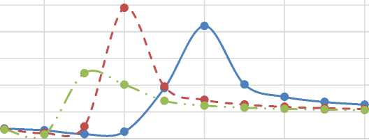
Based on the results of the calculation, the graphs of the amplitude frequency response and phase-frequency response and frequency response of the circuit are constructed. Further in these graphs are under construction:

0,600000

0,500000

0,400000

0,300000

0,200000

0,100000

0,000000

A

AjΩ1

AjΩ2

AjΩ3

2          4          6          8          10

Ω, rad/s

Figure 8. Amplitude frequency response

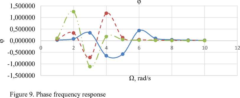
φjΩ1 φjΩ2

φjΩ3

The graphs show a rapid increase in the amplitude A and phase-frequency characteristics φ of the circuit with increasing сyclic frequency Ω from 1 to 6, after which their smooth decay occurs.

For power circuits of the heat transfer calculations are conducted similarly and are written in table 3. A graphical view is presented in graphs 6-7.

The known conditions:

n₀ = 400^

Г1=1ГЁ

(X 1 F

80 x 2

Г kPa • s²l = ^{625 x 10 -3} HH

^ 2

0.002

350 x 2

kPa • s²l = ^2.86X10    | lit |

Г 3

0 2 F

’ 120 x 2

n₀ Q o = — = ^t o

kPa • s²l

=4-17 x 10-3 [—I

400     W

' 100 = 4Й

_ Aq

^{С 1} = t

Q ^- t

a     0.1 x 4              l

- = 057100 = °' ⁰⁰⁸ Ы

C 2 =e 1 = °.°°^[ ₇^ ]

Algorithm for plotting graphs.

The values of the coefficients are calculated:

a 1 = С 1 С 2 Г 1 Г 2 = 0.008 x 0.008 x 6.25 x 10^-3 x 2.86 x 10^-6 = 1.145 x 10^-12               (64)

a 2 = С 1 Г 1 + С 2 Г 1 + С 2 Г 2

= 0.008 x 6.25 x 10-3 + 0.008 x 6.25 x 10-3 + 0.008 x 2.86

x 10-6 = 1 x 10-4

a3 = 1

b 1 = С 1 С 2 Г 1 Г 2 Г З = 0.008 x 0.008 x 6.25 x 10^-3 x 2.86 x 10^-6 x 4.17 x 10^-3 = 4,774 x 10^-15

Ь 2 = С 1 Г 1 Г 2 + С 1 Г 1 Г 3 + С 2 Г 1 Г 3 + С 2 Г 2 Г 3 = 0.008 x 6.25 x 10^-3 x 2.86 x 10^-6 + 0.008 x 6.25 x 10^-3 x 4.17 x 10^-3 + 0.008 x 6.25 x 10^-3 x 4.17 x 10^-3 + 0.008 x 2.86 x 10^-6 x 4.17 x 10^-3 = 4.174 x 10^-7

b₃ = r 1 + r₂ + r₃ = 6.25 x 10^-3 + 2.86 x 10^-6 + 4.17 x 10^-3 = 1 x 10^-2

The limit of change П is accept, П = 1™10 rad/s. Calculation of the real and imaginary part of the frequency function: П = 1 rad/s

Яе(1) =

-a₁b₁^⁴ + (a₃b 1 — a₂b₂ + a₁b₃)^² — a₃b₃ (— a 1 Q² + a 3 )² + a 2 Q²

— 1.145 x 10^-12 x 4.774 x 10^-15 x 1⁴ + 1 x 4.774 x 10^-15 — 1 x 10^-4 x 4.174 x 10^{-7 (}         +1.145 x 10^-12 x 1 x 10^-2

— 1 x 1 x 10-2

)x12

[(—1.145 x 10^-12 x 1 2 + 1) 2 + (1 x 10^-4)² x 1 2 ]

= —0.010425

,      (a^ - a 2 bi)Q 3 + ^b ^ - a^Q, Im(1) =1 (-a1Q2 + a3)2 + a ^ Q2 -(1.145 X 10-12 X 4.174 X 10-7\   13‘ V -1 X 10-4 X 4.774 X 10-15  ' + (1 X 10 -4 X 1 X 10"2 ) V -1 X 4.174 X 10-7 /

66)

₌ _L__________ X 1 __________ J

[(-1.145 X 10^-12 X 1 2 + 1) 2 + (1 X 10^-4)² X 1 2 ]

= 6.255 X 10-7

4(1) = V^(1)² + /m(1)² = ^(-0.010425) 2 + (6.256 x 10^-7)² = 0.010425               ⁶⁷⁾

Im(1)          6.256 X 10-7

„(1) = -arctg ^ = -arctg -0.010425 = 5.99995 X 10"

According to equation write the formula for

RECEIVED INFORMATION FOR HEAT TRANSFER

Table 4

kPa •s 2	kPa • s2]	kPa • s2]	<4-1
r 1 , [     lit    J	r 2 ,[    lit    J	r 3 , [    lit    J	C 1 , Is • o	c 2 , Is • О
0.006251	2.86×10-6	4.17×10-3	0.008	0.008
0.06251	2.86×10-6	4.17×10-3	0.008	0.008
0.006251	2.86×10-6	4.17×10-3	0.08	0.08

The dependency graph is drawn based on input values. For optimal graph perception, take only those values that affect dependencies. The obtained values for the first stage of heat transfer are shown in Table 4.

VALUE AMPLITUDE FREQUENCY RESPONSE FOR ENERGY CIRCUIT

Table 5

Ω	4/121	„j/21	4j/22	„7122	47123	„7'123
1	0,010425	5,99995E-05	0,066684	9,37601E-04	0,010425	1,19999E-04
2	0,010425	1,19999E-04	0,066684	1,87520E-03	0,010425	2,39998E-04
3	0,010425	1,79998E-04	0,066684	2,81279E-03	0,010425	3,59997E-04
4	0,010425	2,39998E-04	0,066683	3,75038E-03	0,010425	4,79996E-04
5	0,010425	2,99997E-04	0,066683	4,68796E-03	0,010425	5,99994E-04
6	0,010425	3,59997E-04	0,066683	5,62553E-03	0,010425	7,19993E-04
7	0,010425	4,19996E-04	0,066682	6,56309E-03	0,010425	8,39992E-04
8	0,010425	4,79996E-04	0,066682	7,50064E-03	0,010425	9,59990E-04
9	0,010425	5,39995E-04	0,066681	8,43817E-03	0,010425	1,07999E-03
10	0,010425	5,99994E-04	0,066681	9,37568E-03	0,010425	1,19999E-03

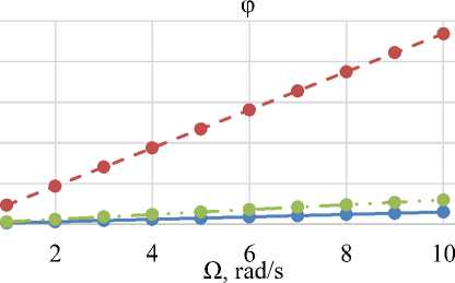
From the power loop heat transfer simulation plots, it can be observed that the amplitudefrequency response of the hydraulic loop A does not change with increasing сyclic frequency Ω, while the phase-frequency response φ increases in direct proportion to its increase.

A

0,08

0,06

<0,04

0,02 — . - --•——•—•—•—•--■•

0,00

0         2         4         6         810

AjΩ1

- • - AjΩ2

—•■ • AjΩ3

Ω, rad/s

Figure 10. Amplitude frequency response

0,010000

0,008000

0,006000

э- 0,004000

0,002000

0,000000

φjΩ1

- • - φjΩ2

—•■ ■ φjΩ3

Figure 11. Phase frequency response

Results and Discussion

The main results obtained from this work are as follows:

A constructive scheme of the experimental setup for the organic Rankine cycle is proposed, and its operating principle is described in detail. The energy circuit of the setup is composed.

Complex impedance, frequency function, amplitude-frequency, and phase-frequency characteristics are obtained through mathematical transformation of the energy circuit. The frequency response of the circuit is constructed.

Modeling of the hydraulic and thermal circuits of the experimental setup is carried out based on the theory of energy circuits.

In the process of modeling the hydraulic energy circuit, it is found that there is a rapid increase in the amplitude-frequency and phase-frequency characteristics of the circuit with increasing cyclic frequency Ω, followed by a smooth decay.

When modeling the heat transfer energy circuit, it is established that the amplitude-frequency response of the hydraulic circuit does not change with increasing cyclic frequency Ω, while the phase-frequency response increases in direct proportion to its increase.

Based on the calculations performed, it is concluded that for the considered scheme of the organic Rankine cycle, the best variant of circuit parameters will be the one in which the hydraulic compliance l2 is twice higher than the initial l1, the cyclic frequency Ω is equal to 4 rad/s, and the active resistance r1 is the largest compared to other calculation variants of r1.

The obtained results are important for predicting the behavior of the experimental setup of the organic Rankine cycle and optimizing its parameters before conducting physical experiments. The proposed approach and modeling methodology have practical value for the analysis and design of similar energy systems.

Conclusion

In summary, this work presents a novel and comprehensive approach to modeling and analyzing hydraulic and heat transfer processes using energy circuit theory, differential equations, and black-box modeling. The proposed methodology integrates these techniques into a unified framework, providing a systematic approach to model development and analysis.

The results obtained from the modeling of the hydraulic and heat transfer energy circuits provide valuable insights into the behavior of the experimental setup of the organic Rankine cycle. The conclusions drawn from the calculations can be used to optimize the circuit parameters and predict the system's performance before conducting physical experiments.

The practical significance of this work lies in its potential to enhance the design and optimization of energy systems involving hydraulic and heat transfer processes. The proposed approach and methodology can be applied to similar systems, facilitating their analysis and improvement.

Further research could focus on validating the model through experimental studies and extending the methodology to other types of energy systems. Additionally, the integration of advanced optimization techniques with the proposed framework could lead to more efficient design and operation of hydraulic and heat transfer systems.

Acknowledgements: Kudaschev Sergei Fedorovich, Zhang Qiang and Levtsev Alexey Pavlovich for for assistance in conducting the research and organizing the article.