Modeling of unidirectional radiation of microdisk resonators with small piercing holes by Galerkin method with accurately computed matrix elements

In the visible and infrared light ranges, dielectric microsize scatterers represent examples of scatterers with configurations exhibiting both geometric-optical (beam-like) and mode effects. The best known such scatterers are lenses of various shapes. In particular, a circular-cylindrical rod and a spherical dielectric particle can concentrate a field of an incident plane wave into a narrow elongated focal spot, usually called a Photonic Jet (PJ) [1, 2] , on the shadow side. Similarly to any focusing effect, PJ is broadband (i.e. not resonant) and has a geometric-optical origin [3] . Moreover, if the frequency or radius of a sphere or rod increases, the PJ region decreases, while the maximum field amplitude in this region linearly increases. However, in addition to the PJ effect, in confined dielectric structures eigenmode resonances are usually easy to notice. In particular, circular dielectric rods and spheres are known to support whispering gallery (WG) modes, which have ultra-high Q-factors that grow exponentially with the mode azimuthal index and radius. When a WG mode is excited by a plane wave, the near-field diagram exhibits azimuthally periodic hot spots along the cavity rim, in addition to the focal region of PJ. Therefore, WG modes corrupt the focus at discrete frequencies.

According to the reciprocity theorem of the electromagnetic field theory, if a point source is placed at the point of maximum field amplitude of PJ, “the inverse PJ effect” can take place. This implies that in a direction opposite to the direction of the plane wave propagation in the scattering configuration, an intense lobe of radiation arises [4 , 5] . This “inverse” effect is also broadband, and the said intense radiation lobe is sharpened, if the optical size of the scatterer increases. At discrete frequencies, however, the beam collimation effect is destroyed by the excitation of WG modes. This occurs because of many equally intense lobes flaring out in the far-field diagram.

It is known that the PJ appears outside the circular scatterer, if the refractive index ν value is smaller than 2. In the opposite case, when ν is large enough, the focal region shifts inside the scatterer [1 –3] . This observation suggests that placing small scatterers in the maximum field of the focal region of a high refractive index microdisk laser can be used to enhance the directivity of radiation of WG modes.

Thin circular microdisk lasers mounted on a pedestal or lying on a low-index substrate are known as microdimensional sources because of their ultra-low WG mode thresholds [6] . They are usually made of high-index materials such as GaAs ( v = 3.4 ). However, their directivity is low because of the large number (twice the azimuthal mode index) of identical lobes in the far-field diagram. This disadvantage of circular microdisk lasers prompted a search for the best shape possible. Among the most promising shapes considered were limacon, serpentine and spiral [7 –9] . To date, there is a consensus that deviations from the circular shape should not be significant so as not to kill the high Q-factors of WG modes. In this sense, a sharp step on the rim of the spiral cavity kills the Q-factor, which outweighs the improvement in directivity. Nevertheless, it should be emphasized that almost all publications (with the exception of the snake shape case [8] ), devoted to the optimal shape search, were based on the analysis of modes in the passive resonator, for which the presence of the active region was ignored.

In the present paper, we are interested in controlling the characteristics of WG modes with the use of a small circular hole. We expect that the hole can improve the directivity of WG modes and keep the generation thresholds low, as it was first proposed in [10] . Our robust computational tool is a set of Muller boundary integral equations (BIE) in a two-dimensional microcavity laser model, whose geometry is shown in Figure 1 . It is considered in the framework of the Lasing Eigenvalue Problem (LEP) proposed for dielectric cavities with active material without loss elements [11] , as well as with loss elements [12] . In the LEP framework, the eigenvalues are modified in such a way that each represents a pair of real numbers being, respectively, the frequency and threshold of radiation generation. Using Galerkin’s discretization method with a trigonometric basis for Muller’s BIE [13] and considering the presence of a symmetry line [14] , we obtain an algebraic eigenvalue problem. The convergence of this numerical method with respect to the matrix truncation number is fully justified mathematically, see [15] ; the details of the algorithm are presented in [16 , 17] .

Preliminary results, significantly more fully disclosed in this paper, were reported at a scientific conference and published in its proceedings [18] .

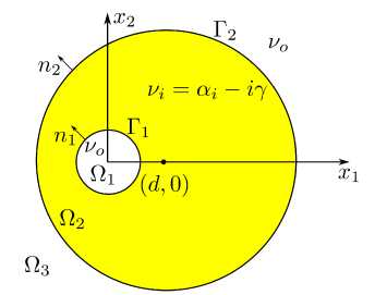
Figure 1. Geometry of a two-dimensional circular dielectric microresonator with a hole

• 1.    Eigenvalue Problem for a Microresonator with a Hole

Following [8] , let us formulate the eigenvalue problem for a twodimensional dielectric circular microresonator with a hole. Let the refractive index in the region Ω 1 (see Figure 1) bounded by the contour Γ 1 be known and positive, which we denote by ν _o > 0 . Let the resonator region Ω ₂ be the active region bounded by contours Γ ₁ and Γ ₂ . The refractive index in the active region is ν i = α i - iγ , where α i > 0 , γ > 0 is the thre shold ga in. The refractive index of the outer unbounded region Ω 3 = R ² \ Ω ₁ ∪ Ω ₂ is equal to the refractive index of the environment ν o > 0 .

We assume that the boundaries Γ ₁ and Γ ₂ are two continuously differentiable closed curves not touching each other. We denote the unit vector of the external normal to the boundary Γ i by n i , i = 1, 2 . Next, we denote by the symbol U the space of all complex-valued functions continuous in Ω 1 , Ω 2 and Ω 3 , and twice continuous differentiable in the open regions Ω 1 , Ω 2 and Ω 3 .

Let the value of the parameter γ > 0 be fixed. The nonzero function u ∈ U will be called the eigenfunction of the problem corresponding to the eigenvalue k > 0 , if one satisfies the following relations, which include the Helmholtz equations:

• (1)    Au + k 2 u = 0, x E Q 1

• (2)    Au + k ² u = 0, x E Q 2 ,

(3)                     Au + k 2 u = 0, x E П 3

conjugation conditions:

(4)	u = u + , n o ju— ∂n 1	∂u + = n i dn ;	,x	E Г ;
(5)	u - = u + , n i Ju— ∂n 2	∂u + = no я— ∂n 2	,x	E Г 2
and the Sommerfeld radiation condition:
(6)	( It - ik o ^u = ∂ρ	o ( tp ) •	ρ →	∞ .

Here k j = kv j is the wave number in the corresponding region; n j = v - ² in the case of H -polarization and n j = 1 in the case of E -polarization; j = i, o ; u - (u + ) are the limit values of the function u from inside (outside) the contour r i ; i = 1,2 .

Following [19] , p. 68, we assume that the limit values of the (proper) normal derivative

∂u ^±

• (7)    ——( x) = lim (n i (x), gradu(x ± hn(x))), x E r i , i = 1, 2, ∂n _i       h → +0

exist uniformly along x on r i , i = 1, 2 .

We will search for nontrivial solutions of the problem (1) - (6) in the space of complex-valued functions U . At a fixed value of the parameter y > 0 , the nonzero function u satisfying the Sommerfeld radiation condition will be called the eigenfunction of the eigenvalue problem for a circular dielectric microresonator with a hole, corresponding to the eigenvalue к >  0 , if the conditions (1) - (5) are satisfied.

u=

f ⁽ dG o (k; x,y) J г Д ^dn i ⁽ y)

^{u (} y ^{) -}

^- G _o ⁽ k; x,y) ^du ^{( y )} )dl⁽y⁾, dn i (y)

x E fi i ,

• (9)    u = ( ( ^dGi(^k,Y^;x^,y) u + (y) - G i (k,Y; x,y)д^Adly)-rP   dn i (y)                       dn i (yP

  
  

[ ( ^{дG i} ( ^k,Y' ^, X,^y) u - (y) - G i (k,Y; x,y) dm )dl(y), x e П 2 , J r2^V    dn 2 (y)                         dn 2 (yp

• (10)    u = / ( ^dG o ^(k;x^,y) u + (y) - G o (k; x,y)lu + y) ) dl(y),  x e П 3 ,

r ₂V dn 2 (y)                         дп 2 (у)

where G j (x,y) = (i/ 4)H ⁽¹⁾ (k j | x - y | ) , j = i, o , H ⁽¹⁾ is a Hankel function of order zero.

Using the conjugation conditions (4) and (5) , we define the functions

(11)	U j = u + = u , x e r j ,   j = 1, 2,
(12)	= n i + П о du + = n i + П о du -        Г 1       2n o dn 1        2n i dn 1 ,     e 1 ,
(13)	= n i + П о du + = n i + П о du -        Г V2       2n i dn 2       2n o dn 2 , X E 2.

Let us add term by term the limit values of the integral representations (8) - (10) and their normal derivatives on both sides of the contours Г 1 , Г 2 , using the well-known properties of simple and double layer potentials (see, e.g., [19] , p. 47). Thus, we obtain a homogeneous system of Muller boundary integral equations with respect to the functions u and v :

• (14)    upp+f ui(y)K1,1(x,y)dl(y)+ [ vi(y)K1,2(x,y)dl(y)+ Γ1

+ [ u2(y)Ki3(x,y)dl(y)+ [ v2(y)Ki4(x,y)dl(y) = 0, x e Г1 Γ2

• (15)    vi(x)+ [ ui(y)K2,1(x,y)dl(y)+ [ vi(y)K2,2(x,y)dl(y)+ Γ1

+ [ U2(y)K2,3(x,y)dl(y) + [ v2(y)K2,4(x,y)dl(y) = 0, x e Г1, Γ2

• (16)    u2(x)+[ ui(y)K3'1(x,y)dl(y)+ [ vi(y)K3,2(x,y)dl(y) + Γ1

+ / u2(y)K3,3(x,y)dl(y) + [ ^(y^K^xyWy) = 0, x Е r2, Γ2

• (17)    v2(x)+ [ ui(y)K4,1(x,y)dl(y)+ [ vi(y)K4,2(x,y)dl(y) + Γ1

• 3. Galerkin Method

+ [ u2(y)K4,3(x,y)dl(y)+ [ v2(y)K4,4(x,y)dl(y) = 0, Γ2

x Е Г 2 ,

where the kernels of the integral equations have the form

(18)	K ^' 1 =	dG o (x,y) - дG г (x,y)     _ r     _ dn i (y)       dn i (y) , X      1 ,У	г 1 ,
(19)	K 1, 2 =	,    GGx,y:        ,    Go (x,y), x П г + П о            П г + П о	Е г 1 ,у Е г 1 ,
(20)	K ^' 3 =	^г^У) dn 2 (y) ’ x € Г 1 ,у € г 2 ,
(21)	K 1 ’4 =	2n o G г (x,У) , x € г 1 , y € Г 2 , П о + П г
(22)	K2'1 =	д 2 G o (x,y)      д 2 G i (x,y)     x €	г 1 ,у Е г 1 ,
		dn 1 (x)dn 1 (y) дп 1 (х)дп 1 (у) ’
(23)	K2'2 =	2n o dG i (x, у)      2п г dG o (x,y)	x Е г 1 ,у € г 1
		n o + П г dn i (x)      n o + П г dn i (x) ,
(24)	K 2'3 =	д 2 G г ( x,У )
		Я                \ , x € Г 1 , y € Г 2 , дп 1 (х)дп 2 (у)
(25)	K2'4 =	2n o дG г (x,y) 1       я Г \ , x € г 1 , у € г 2 , n o + П г дП 1 (х)
(26)	K 23'1 =	дG г ( x,У ) дп 1 (у) , x € г 2 ,у € г 1 ,
(27)	K 23'2 =	2n o G г (x,У) , x Е г 2 , у € г 1 , n o + П г
(28)	K 23'3 =	дG г (x,y ) _ dG o (x,y)     Е г Е дп 2 (у)       дп 2 (у) , Ж      2 ,у	г 2 ,

146	I. V.	Ketov, A. O. Spiridonov, A. I. Repina, E. M.		Karchevskii
(29)	K ' =	G o (x,y)	2n o -     ,     G i (x,y), x	€ Г 2 , y € Г 2 ,
		n + П о	П г + П о
(30)	K 24 , i =	d 2 G i (x,y)	x € Г 2 ,У € P i ,
		dn i (y)dn 2 (x)’ 2n o dG i (x, y)
(31)	K 24 , 2 =		, x € P 2 ,y € P i ,
		П о + n i dn 2 (x)
(32)	K 24 , 3 =	d 2 G i (x,y)	d 2 G o (x,y)        €	Г 2 , y € Г 2 ,
		dn 2 (x)dn 2 (y)	dn 2 (x)dn 2 (y),
(33)	K 24 , 4 =	2пг dG o (x,y) П о + П г dn 2 (x)	-   2n o dG i (x,y) П о + П г dn 2 (x) ,	x € Г 2 , y € Г 2

Let the contours Гi and Г2 have the form of circles of radii ai and a2, respectively. We obtain explicit expressions for the matrix elements of Galerkin’s method. In (14)-(17), let us perform the substitutions wi(t) = aiui(t),   W2(t) = aivi(t),   W3 (t) = a2U2(t),   W4(t) = a2V2(t).

We will search for approximations to functions w k (t) in the form of Fourier series segments of the form

n

Wk(t) = V wmk)Фm(t),   k = 1,2, 3, 4, m=^

where ^ = 0 , if ф _m (t) = cos(mt) , m = 0,..., n, are used as basis functions and ^ = 1 , if ф _m (t) = sin (mt) , m = 1,..., n are used as basis functions. We define the scalar product as

2n

^{( u,v )} = 2n j ^{u ( t ) v ( t ) dT}, 0

u, v € L ₂ .

Applying Galerkin’s method, we obtain a system of linear algebraic equations

¹    (i)

w a ^l

nnn

+ V h⁽ⁱ,ⁱ⁾w(i) + V /W²» + V h⁽ⁱ,³⁾w(3) +

⁺ / , hlm w m ⁺ / , hlm w m ⁺ / , hlm w m ⁺ т=д          m=^          m=^

n

⁺ E h Vr^ w m = °, l = M,...^,n, т=д

(37)	1    (2) w a i l	+	n ∑︂ т=д	(2, ) h lm	( ) w m	+	5" /l(2 , 2)w(2) h lm w m т=д	n + e h !rn,” w s:| + т=д
							n + E h l;:4) т=д	(4) *-ит        ,	l = ц, . . .	,n
(38)	1    (3) w a 2 l	+	n ∑︂ т=д	(3, ) h lm	( ) w m	+	E /l(3 , 2)w(2) h lm w m т=д	n + E h (.“) w £3) + т=д
							n + E h irn , 4) т=д	(4) w .     ,	l = ц, . . .	,n
(39)	1    (4) w a 2 l	+	n ∑︂ т=д	(4, ) h lm	( ) w m	+	E n    (4,2) (2) h lm w m т=д	n + E h !i,” w £!l + т=д

n

+ E h^wm = °, l = M,.--,n- т=д

The Galerkin method matrix is a second-order block matrix. The elements of the upper left block have the form hj _ z / / 7>-i,j i i      iAm,(tiAdTidti m, l = ц,... ,n,

m, l = ц, .. ., n,

m, l = ц, .. ., n,

hlm = п у J Ki (t1,T1 )фmVтi )фl\ti)dтi dti, where i, j = 1, 2.

The elements of the upper right block have the form

2п /*2п

^т^ = ~          Kl’j (t2,T2!)фm(T22)фl(ti)dт22dti, n Jo Jo where i = 1, 2, j = 3, 4.

The elements of the lower left block have the form z     2n 2n _ , „ ,          . ------„ h^ =               KJ (ti,тi')фm(тi')фl(t2>)dтidt2, n 0    0

where i = 3, 4 , j = 1, 2 .

The elements of the lower right block have the form п     2п   2п . - „ „         „ -------- „ „ m, l = ц, .. ., n,

him =—      K2 (^Т^ФтХт^ф/^Ж^, п Jo  Jo where i, j = 3, 4. Here nl = 1/2, if l = 0, and nl = 1, if l = 0.

Let the distance between the centers of the circles Г 1 and Г ₂ be d , and the radii of the circles be a 1 and a ₂ , respectively. Then the matrix elements of Galerkin’s method, according to [20] , have the form:

h^ ’¹) = ук _о^ (к _о а 1 )Н _г ⁽¹⁾ (k ° a/ - yAJ i^ a^H ¹) (k ₄ a i ),

h(1,2) = inn° Ji(kia1)H(1)(kгa1)--innL_Ji(k°a/H(1)(k°a1), Пг + П°           l            Пг + П°            l h^3) = ^ kiH^1)’ (kia2)(Jm-i(kir)Ji (kia1)(-1)(m-l) +

+ J _{m +}i (k i r)J - i (k г a 1 )( - 1) ^{( m + l +}^⁾ ) ,

h (m⁴⁾ = - i^"'" H «(^J m - i (k i r)J i (k i a 1 )( - 1) ^{( m-l )} + n ° + П г

+ J m+l (k i r)J - i (k i a 1 )( - 1) (^{m+l +}^ ,

LI2,1)   ink° '            (1)‘             inki ‘           (1)‘ hll           2 Jl \k°a1)Hl    \k°a1)      2 Jl \kia1)Hi    (kial),

h ⁽2 ^{, 2)} = — + i ⁿⁿ ° k i J i (k i a 1 )H ⁽¹⁾ (k i a 1 )

• ^ll a 1     П г + П °               l

• ^{1    ПП г} k ° J l (k ° a 1 )H ⁽¹⁾ (k ° a 1 ), П г + П °

h ^{( 2} m ³ = inn l k г² H m¹⁾ ‘ (k г a 2 ) ( J m - l (k г r)J l ‘ (k г a 1 )( - 1) ⁽m -^{l )} +

+ J m+l (k г r)J - l (k г a 1 )( - 1) ^{( m + l +}^⁾ ) ,

h (m,⁴⁾ = - Пг +7 k г H m¹⁾ (k г a 2 ) ( J m - l (k г r)J l ‘ (k г a 1 )( - 1) ⁽m -^{l )} +

+ Jm+l (kгr)J-l(kгa1)(-1)(m+l+^)), hl(m,1) = - innl kгJm (kгa1 )(Hl(kгa2)Jm-l (kгr)

+ (-1)мн-l(kгa2) Jm+l(kгr)), hm2 = ПЛ+П;1 Jm (kiai)(Hl(kia2)Jm-l (kir)

O +(-W-l (kia2)Jm+i(kir)), hu'3 = inkiJi(kia2)Hl(1) №«2) - i-^kJJi(koa2)H(1 (koa^),

h(t’4 = -i^i- Ji(koa2 )H(>4koa2) — -^J Ji (^H^(W, П + no       '            n + По         l h^1 = — i2^ J (kiai)(Hi(1)‘ (kia2)Jm-i(kir)+

+ ^{( —} 1 ^{) M} H — ^(k i ^a 2 ) ^J m+i ^(k i r)^ ,

h ⁽m² = -i^J⁰ k i J m (k i a i )(H ⁽¹⁾ ‘ (k i a 2 )J m - i (k i r)+ H i + П о

(-l^H-1) (kia2)Jm+i(kir)), hu'4 = inki2Ji‘(kia2)H(1)‘(kia2) - i^k^Ji’(koa2)H(1)‘(koa2), h(4,4) = — + ^^^^koJi(koa2)H(1) (koa2)- ii       a2    Hi + Ho               i inno ki j(kia2)H(1)(kia2), Hi + Ho              i where m,l = ц,... ,n, oi = 1 /2, if l = 0, and oi = 1, if l = 0.

( a ) D in H-polarization

( b ) γ in H-polarization

О -----------------'------------------------'------------------------'------------------------'------------------------'------------------------'------------------------'------------------------

О 0.1   0.2   0.3   0.4   0.5   0.6   0.7   0.8

d

( c ) D in E-polarization

( d ) γ in E-polarization

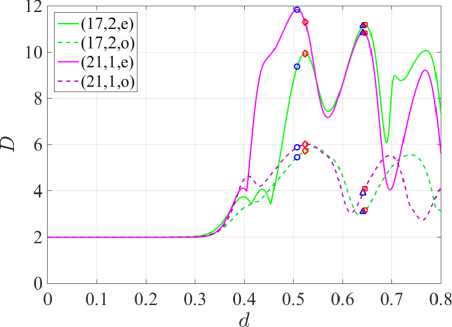
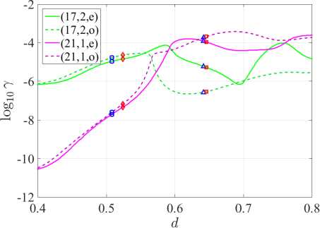
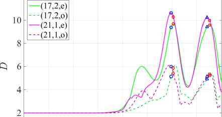
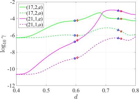
Figure 2. Dependences of directivity D and radiation generation threshold γ on d

denote each mode by the same indices as in the limiting case d = 0 . Note that for larger values of d , these notations may become less obvious.

In our calculations, we investigate the behavior of H- and E-polarized quasi-WG modes, for which the normalized frequencies at d = 0 differ in the 3rd place for the H-polarization case, and in the 2nd place for the E-polarization case. Namely, in the case of H-polarization we have the following initial points at d = 0 : к = 9.9924, 7 = 6.07232 x 10 ^{- 7} and к = 9.9948,7 = 2.01306 x 10 ^{- 11} for doubly degenerate modes (17, 2) and (21, 1) respectively. In the case of E-polarization at d = 0 : κ = 9.6112, γ = 5.01117 x 10 ^{- 7} and к = 9.6239,7 = 2.13596 x 10 ^{- 11} for the same (17, 2) and (21, 1) modes, respectively. The hole radius normalized to the radius of the microdisk is fixed at r = 0.03 . We are interested in obtaining the maximum radiation directivity D accompanied by a relatively small value of the generation threshold γ (see Figure 2) .

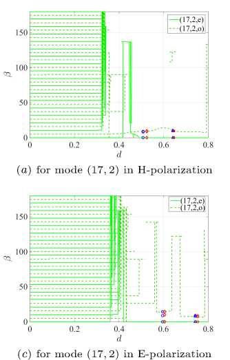
Figure 3. Dependences of the angle β of maximum directivity on d

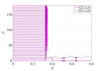
( b ) for mode (21, 1) in H-polarization

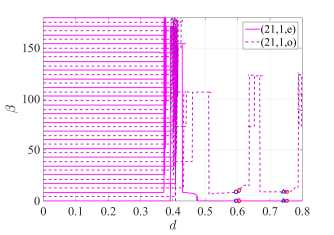
( d ) for mode (21, 1) in E-polarization

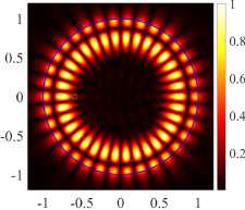
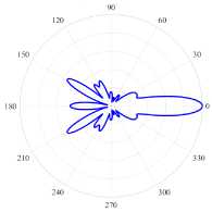
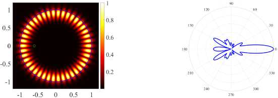
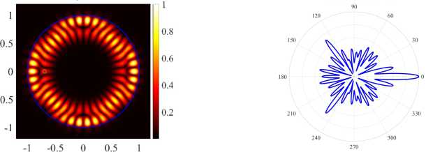
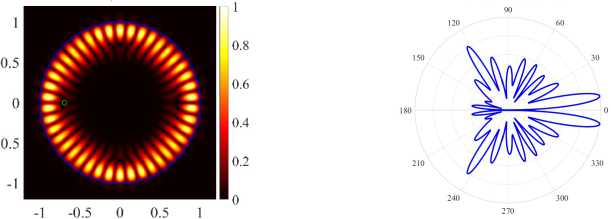
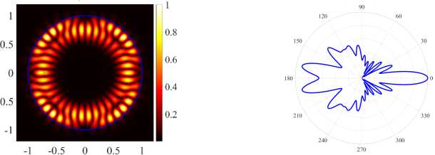
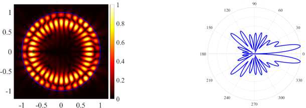
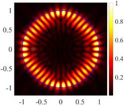
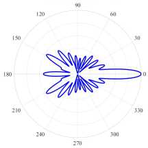
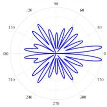
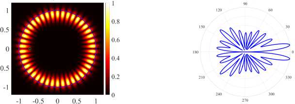
The definition of D is given in [13] (see equation (46)). The Figure 3 help control the direction of the main lobe in the far-field diagrams (see right panels in Figure 4. The blue markers in Figure 2 and Figure 3 correspond to the first and second mode directional maxima (21,1,e) , whereas the red markers correspond to similar mode maxima (17, 2, e) . For detailed analysis, we select the first D mode (21,1, e) maxima, see Figure 4 in the case of H-polarization and Figure 5a in the case of E-polarization. In the case of H-polarization, at d = 0.51 we have the greatest directivity for the (21,1, e) mode, accompanied by a relatively small threshold 7 . The threshold of this mode is the lowest among all four studied modes, and their normalized frequencies differ in the third sign. In the case of E-polarization at d = 0.599 the normalized frequencies of the studied modes differ in the second sign, and the mode (21,1, e) has the greatest directivity, but the threshold of the mode (21,1, o) is lower than that of the mode (21,1, e) .

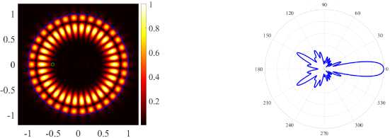
( a ) (17, 2,e), k = 9.9927, log ₁₀ (7) = - 4.9457, D = 9.51

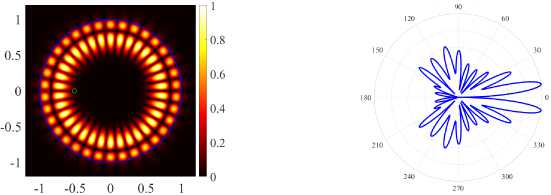
( b ) (17, 2, o), k = 9.9929, log ₁₀ (7) = - 4.7586, D = 5.50

( c ) (21, 1, e), k = 9.9948, log ₁₀ (7) = - 7.6640, D = 11.83

( d ) (21, 1, o), k = 9.9948, log ₁₀ (7) = - 7.5550, D = 5.90

( a ) (17, 2, e), k = 9.6229, log ₁₀ (y ) = - 3.9864, D = 8.21

( b ) (17, 2, o), k = 9.6138.5, log ₁₀ (y ) = - 5.1499, D = 4.25

( c ) (21, 1, e), k = 9.6313, log ₁₀ (y ) = - 2.9738.5, D = 9.23

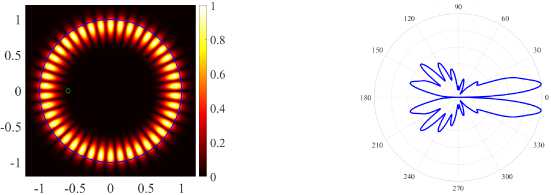
( d ) (21, 1, o), k = 96241., log ₁₀ (y ) = - 6.3621, D = 4.47

( a ) κ in H-polarization

( b ) γ in H-polarization

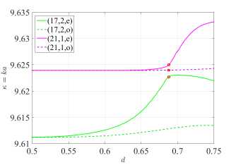
( c ) κ in E-polarization

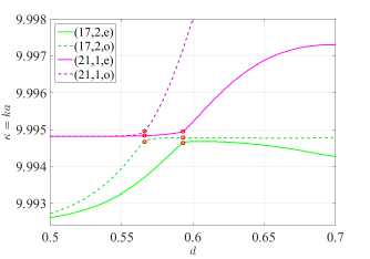
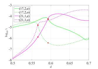
Figure 6. Normalized frequency κ and emission threshold γ vs. hole offset d

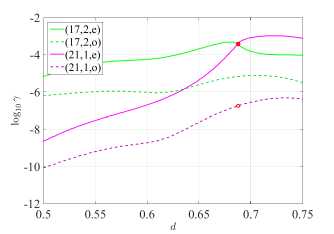
( d ) γ in E-polarization

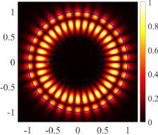
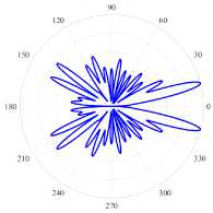
Both in the case of H-polarization at d = 0.51 and in the case of E-polarization at d = 0.599 , we obtain quasi-singular radiation for each of the modes of even type. Odd-type modes have two equally intense lobes at a smaller value of the directivity coefficient D . Increasing d , we obtain the K(d) and y (d) plots shown in Figure 6. The right panels for y (d) represent an increase in the [0.5, 0.7] and [0.5, 0.75] segments of right panels of Figure 2 for H- and E-polarizations, respectively. Note that the values d = 0.51 and d = 0.599 lie before the “avoided resonance crossing” effects for the corresponding polarizations.

When the frequencies of the (17, 2, e) and (17, 2, o) modes begin to grow and approach the frequencies of the (21,1, e) and (21,1, o) modes, respectively, we observe the “avoided resonance crossing” effect in Figure 6. More precisely, the frequencies of modes avoid crossing, but the γ generation thresholds do actually cross (see right panels of Figure 6) .

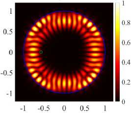
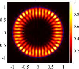
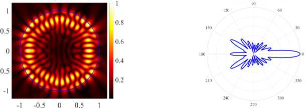
Let us consider in detail the points at which the frequencies avoid intersection. For H-polarization: d = 0.566 and d = 0.592 (see Figure 6a and Figure 6b), whereas for E-polarization: d = 0.688 (see Figure 6c and Figure 6d). For each two-component eigenvalue (к, y), we have two orthogonal eigenmodes (odd and even). In [21], it was suggested that “pseudo lattice modes” appear if eigenvalues of two or more modes belonging to different azimuthal families approach each other (in frequency) in the (Re к, Im к) plane. The same can be expected in the LEP analysis as well, in the (к, y) plane. It is also known that when two eigenvalues are close to each other and an “avoided resonance crossing” effect is observed, hybridization of the mode fields occurs [22]. Indeed, for H-polarization there is hybridization of the mode fields (17, 2, o) and (21,1, o) at d = 0.566 (see Figure 7a) and hybridization of the mode fields (17, 2, e) and (21,1, e) at d = 0.592 (see Figure 7). Similarly, for E-polarization there is hybridization of the (17, 2, e) and (21,1, e) mode fields at d = 0.688 (see Figure 7). In further investigation, we observe that the field diagrams in the near zone of the pairs of quasi-embodied modes in the strong coupling region (controlled by the hole displacement parameter, d) acquire shapes approximately equal to the sum and difference of fields of the two considered modes.

Our goal is to achieve quasi-single-directional emission, but we see that the modes under study acquire new properties as a result of hybridization. We call them PJ enhanced WG modes, because of the specific patterns of the near-field diagrams.

Namely, bright spots of the field do not bypass the perturbed region (hole), but concentrate around it. The nature of this phenomenon, which we observe for even modes having field maxima near the hole, can be explained using the PJ effect. In Figure 6b, we see that the thresholds of the (17, 2, o) and (21,1, o) modes intersect at d = 0.566 . Note that the (21,1, e) mode does not participate in hybridization, although its frequency is close to the frequencies of the hybridized modes, since it belongs to the orthogonal symmetry class. Similarly, for E-polarization at d = 0.688 (see Figure 6d) , the thresholds of the (17, 2, e) and (21,1, e) modes cross, and the (21,1, o) mode does not participate in hybridization. The hybridizing modes turn into the sum and difference of two quasi-WG modes.

In the case of H-polarization, at the first point d = 0.566 the odd modes begin to transform into rhomboid and triangular modes (see Figure 7a) ,

(21, 1,o) - (17, 2,o), к = 9.9950, log ₁₀ (Y) = - 4.8057

(21, 1, o) + (17, 2, o) к = 9.944, log ₁₀ (Y) = - 4.8291

1    -0.5    0     0.5     1

( a ) case of H-polarization, d = 0.566

(21, 1,e) - (17, 2, e), к = 9.9949, log ₁₀ (Y) = - 4.2858

(21, 1,o) + (17, 2, o), к = 9.9946, log ₁₀ (Y) = - 4.2099

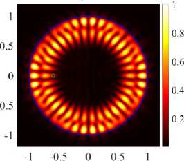
( b ) case of H-polarization, d = 0.592

(21, 1, e) - (17, 2, e)

к = 9.6250, log ₁₀ (Y) = - 3.3909

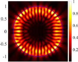
(21, 1,e) + (17, 2, e), к = 9.6227, log ₁₀ (Y) = - 3.4406

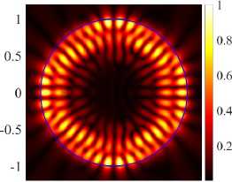
-1    -0.5    0     0.5     1

1    -0.5    0     0.5     1

( c ) case of E-polarization, d = 0.688

whereas at the second point d = 0.592 the even modes begin to transform into square modes (see Figure 7b) . In the case of E-polarization at d = 0.688 , the even modes begin to transform into hexagonal modes (see Figure 7c) . In figures 7b , 7c we observe the penetration of the field into the inner region, the field maxima do not bypass the hole. At all three points where the frequencies avoid intersection, the threshold of one of the modes drops sharply, while the other increases (see Figure 6) .

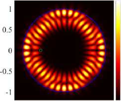
At the points where the frequencies avoid intersection, there is an exchange of fields between the corresponding modes. After the exchange of fields for the H-polarization of PJ, the amplified WG modes (17, 2, o) and (21,1, o) become rhomboid-shaped (see Figure 8) and triangular-shaped (see Figure 8d) . Around the second point for H-polarization, we observe an exchange of fields for even modes (17, 2, e) and (21,1, e) . Similarly, for E-polarization near the point d = 0.688 we observe an exchange of fields between the even modes (17, 2, e) and (21,1, e) . After the exchange of fields, the (17, 2, e) and (21,1, e) modes become rhomboid-shaped (see Figure 9a) and hexagonal (see Figure 9c) . Even modes have higher directivity values; in addition, their radiation is quasi-single-directional, which is confirmed by normalized field diagrams in the far zone.

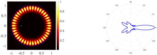
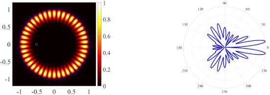
We investigate the eigenvalues and directivity of radiation after the exchange of the mode fields (see Figure 8a for H-polarization and Figure 9 for E-polarization). As a result of our study for H-polarization, we can conclude that the even mode (17, 2, e) (see Figure 8a) has the maximum directivity at the minimum value of the generation threshold at d = 0.694 . In the case of E-polarization, the even mode (21,1, e) (see Figure 9c) has maximum directivity at d = 0.72 , but the threshold of the mode (21,1, o) (see Figure 9d) is less than that of the (21,1, e) mode. The high directionality of the (21,1, e) mode is due to the inverse effect of PJ.

Conclusion

The results of our numerical experiments, performed with a carefully tested software complex, confirm the assumptions of [21 , 22] that the threshold gain and directivity characteristics of a microdisk laser can be controlled with a small hole. Namely, we found that a small hole drilled in the inner focal region of a high refractive index microdisk laser leads to enhanced directivity of the emission of WG modes, while the

( a ) (17, 2, e), k = 9.9943, log ₁₀ (7) = - 6.1656, D = 6.58

( b ) (17, 2, o), k = 9.9948, log ₁₀ (7) = - 6.0355, D = 4.88

( c ) (21, 1, e), k = 9.9973, log ₁₀ (7) = - 4.4054, D = 4.08

( d ) (21, 1, o), k = 10.0211, log ₁₀ (7) = - 3.4314, D = 5.53

( a ) (17, 2, e), k = 9.6229, log ₁₀ (7) = - 3.9864, D = 8.21

( b ) (17, 2, o), k = 9.6134, log io (7) =

- 5.1499, D = 4.25

( c ) (21, 1, e), k = 9.6313, log ₁₀ (7) = - 2.9734, D = 9.23

( d ) (21,1, o), k = 9.6241, log ₁₀ (7) = - 6.3621, D = 4.47

threshold of emission generation remains small. In contrast to [21, 22] , this conclusion is based on classical full-wave electromagnetic field theory and does not use the billiard theory or the concept of wave chaos. Thus, it provides a simple and clear engineering rule for the hole placement.