Моделирование анизотропии галактических космических лучей

The idea of using galactic cosmic rays for monitoring processes in the heliosphere has existed for a long time [Dorman et al., 1995] . Advances in this direction are, however, limited, largely due to the difficulty in calculating cosmic ray trajectories in the interplanetary magnetic field and the difficulty in calculating the magnetic field itself. In this paper, we address this problem using simple model examples, considering anisotropy modeling as a scattering problem, i.e. we assume that all cosmic rays are generated by an isotropic flux incident from infinity. This formulation was proposed, for instance, by Parker [Parker, 1965] .

Note that cosmic ray propagation is generally considered within the framework of the diffusionconvection model when the turbulent scattering is taken into account in addition to motion in the regular electromagnetic field. In particular, the effect of the 22-year solar cycle on the anisotropy of cosmic rays with energies of 10 GeV and higher is examined using this model in [Krymsky et al., 2010] . Also noteworthy is that the anisotropy in Earth’s orbit can be studied without regard for diffusion. In this paper, we consider only the motion in a regular field.

It is known that solar wind plasma in the heliosphere may be thought of as a perfect conductor. This means that the electric field in the local reference frame is zero, whereas in the celestial reference frame it is proportional to a small parameter v /c ~10-3, where v is the solar wind velocity. The time derivative of the magnetic field will be of the same value in the celestial reference frame (so-called condition of magnetic field frozen; see, e.g., [Landau, Lifshitz, 1992], § 65). Hence it is clear that in the Lorentz force acting on cosmic rays,

F = e | E + u x B | ,                            (1)

I c J where u~c is the velocity of cosmic rays, the main term is that with the magnetic field, which can also be regarded as static. The magnetic field variation with time and its associated electric field are corrections. As a first step we, therefore, address the problem of calculating the anisotropy in the static magnetic field.

In this way, we get an impressive general result: the static magnetic field in itself proves to be unable to produce any anisotropy. If an incident flux is isotropic, the angular distribution at any space point will be isotropic.

Thus, the anisotropy is generated by moving field inhomogeneities. This means, firstly, that it is weak, v / c ~10^-3, and, secondly, that the greatest contribution to it is made by the fastest moving inhomogeneities. We examine a model field of a moving magnetic cloud and compute anisotropy at different relative positions of the cloud and observer. This anisotropy is fairly typical: it comprises either one region with increased or decreased flux, or two adjacent regions in one of which the flux is increased, and in the other it is decreased. Similar pictures are observed by the muon hodoscope URAGAN [Yashin et al, 2015] .

TWO-DIMENSIONAL

AXIALLY SYMMETRIC STATIC MAGNETIC FIELD

To obtain an analytically solvable problem, we examine a two-dimensional case. We consider the

This is an open access article under the CC BY-NC-ND license magnetic field as perpendicular to the plane of motion and symmetric under rotation around a center. In polar coordinates associated with the center, this field can be described by the vector potential A (r). Notice that the coronal mass ejection model in the form of a cylinder with a longitudinal or spiral magnetic field inside is quite widely accepted [Burlaga, 1988; Osherovich et al., 1993]. Our aim here is to relate the angular distribution of particles at the observation point with the distribution of incident particles at infinity.

It is most convenient to find cosmic ray trajectories from the (relativistic) Hamilton-Jacobi equation ([Landau and Lifshitz, 1988b] , § 16)

1 Гд5 Y <55 У  Г1 5Sc2 ( 51)   ( 5r )   ( r 5ф

- Aф(r )j = m c .  (2)

Instead of the traditional energy E and momentum

L introduced for the cyclic variables t and ф , it is

convenient to operate with the momentum p = E¹ / c ² — m²c² and the impact parameter a = L / p , then the principle function of the Hamilton-Jacobi equation takes the form

5 = — tsjp^c1 + m2c4 +

and hence the trajectory equation is derived by differentiating with respect to the impact parameter a

^{ф( r} ) = ^ф о ⁺ J r

.

When r →∞, the integral converges, defining an asymptotic direction ф„. The angle 0, at which the trajectory leaves the reference point ( r , ф₀), measured from the azimuth direction, is defined by the equality (Figure 1)

ae cos0 =---A (ro).

r pc

If we now imagine that near the point ( r , ф₀) there is a radially oriented area dr 0 and figure out how many particles are incident on it in the range of angles (θ, θ+ d θ), assuming that the distribution with r → ∞ is known, this problem is solved by calculating the Jacobian from ( r 0 , 0) to ( a , ф „ )

dad ф „

5 a

⁵ r o

5^

⁵ r o

5ф.

dr ₀ d 0 .

However, whereas Formula (5) directly defines a as a function of r 0 and θ, Formula (4) with r →∞ defines ф_ю as a function of r 0 and a , so

5 a5

5 r50

^{5ф 5ф}

5 r50

5фю 5a5r 50

5 a

⁵ r o

5ф„ ! 5ф„ 5a5 r   5 a 5 r

= cos0

and finally

da dф„ = cos0 dr d0.

5 a

5ф„ 5a

5a 50

The factor cosθ takes into account the fact that at oblique incidence the effective area is cosθ dr 0 . Thus, this equality means that at isotropic particle incidence from infinity their distribution over directions at ( r , ф ) remains isotropic. Note that the specific

expression for A ( r ). is missed completely in the result. The next section shows that the result is valid in general for any static magnetic field and in the threedimensional case.

There is one exception here: generally speaking, not any trajectory in the magnetic field must go to infinity. In terms of the scattering problem, in addition to trajectories of passing particles there may be trajectories of trapped particles, which always remain in a bounded region of space (a well-known example is Eart’'s radiation belt). In this case, the boundary condition at infinity is not adequate — to set the distribution over trajectories of trapped particles requires additional considerations. The simplest of them is the assumption about the absence of trapped particles, i.e. the absence of particles on the trajectories that do not run to infinity. Then, in the angular distribution at this point the anisotropy appears which depends on whether only trajectories of passing particls go through this point or trajectories of both passing and trapped particles, or only trajectories of trapped particles (Figure 2). In the first case there is no anisotropy. In the second case, there is a cone of directions corresponding to

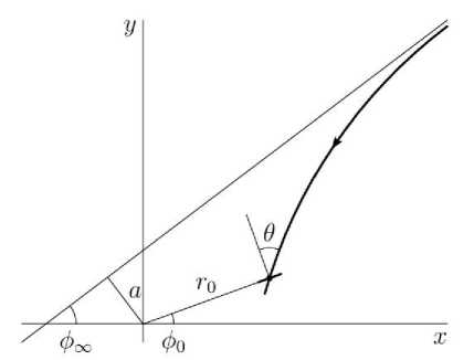
Figure 1 . Coordinates and angles. The magnetic field symmetry center is at the origin. The observation point has polar coordinates ( r , ф₀) . The bold line indicates a small radially oriented area at the observation point and a particle path, θ is the incident angle measured from the normal to the area. Also shown are an asymptotic direction (at an angle ф_т ) and an impact parameter a

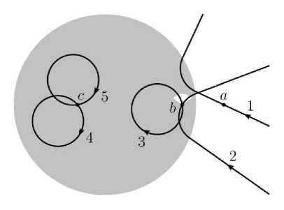
Figure 2 . Passing and trapped particles. In the gray area, the magnetic field is homogeneous, and is absent outside. Through a , trajectories of only passing particles (1) run; through b , trajectories of both passing (2) and trapped (3) particles; through c , trajectories of only trapped particles (4, 5). The cone of directions of the trapped particle trajectories at b are shown in white

trajectories of trapped particles, in which there is no flux; in addition to the cone the flux is the same as in the first case (thus, the total flux decreases). In the third case, the flux is zero in any direction.

If incident particles have not one fixed energy but energy distribution, the above picture is smoothed, but remains qualitatively similar: in the area of coexistence of passing and trapped particles there appear a cone of directions with a reduced flux. Energy distribution of recorded galactic cosmic rays over a wide region can be described by the formula

dN dE

--2.7

~

0,

' min ,

'min’

here E min is the cutoff energy of a recorder.

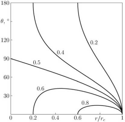
Figures 3 and 4 plot anisotropy due to capture of particles in the two-dimensional model problem with a potential

А ф ( r ) =

( r - r c ) B /2, 0,

r <  r c ,

r >  ^r c -

Figure 3 . Cone apex angle of trapped particles as a function of distance from the center of magnetic field symmetry for different values of the ratio r _g/ r _c (indicated near curves in the Figure), r _g is the particle gyroradius, r _c is the radius of a region with a homogeneous magnetic field

This potential refers to a homogeneous magnetic field in the region r < r c . As known, in the homogeneous magnetic field a particle moves in a circle of radius

r _g = pc /( eB ),

(so-called gyroradius) particles can be trapped if r g / r c <1. A similar condition remains qualitatively valid for an arbitrary field: particles can be trapped if the area occupied by the field is larger than the double gyroradius in this field.

ABSENCE OF ANISOTROPY IN AN ARBITRARY STATIC MAGNETIC FIELD

The above conclusion, drawn for the special case, about the absence of anisotropy is in fact quite general and is associated, on the one hand, with phase volume conservation when the Hamiltonian system is moving, and, on the other hand, with constant particle velocity in the static magnetic field.

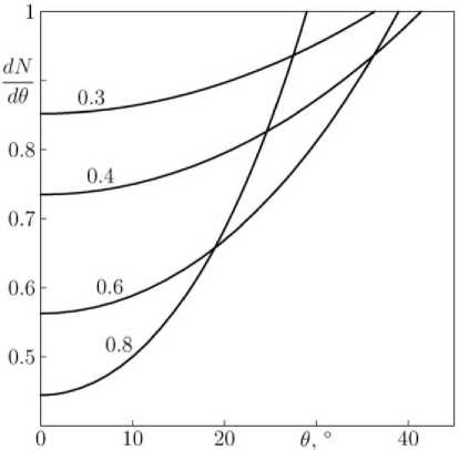
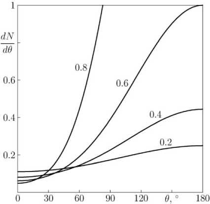
Figure 4 . Angular dependence of a flux in the case of energy distribution of particles ~ E ^–3 at different distances (indicated on curves) from the field center. Gyroradius of minimum energy particles r _g/ r _c=0.2 for panel a and r _g/ r _c=0.6 for panel b

Suppose we have a system with a Hamiltonian H ( p , r , t ) and that n ( p , r , t ) is the phase density, the number of particles in given intervals of coordinates and momenta at a given time in our case. This number of particles can be converted to a flux through an area dS in a solid angle d Ω as follows:

dN = n(p, r, t) d2 p d3 r = d3 u

= n ( p , r , t ) —------------ u dS dt =              (12)

| d ² H / d p d p_} |

, u³ du d П dS dt

= n ( p , r , t )                    ,

| d2 H / dpdp} | where | 62 H / 6p, dp. |=| 6u, / 6p. | is the Jacobian from momenta to velocities u = dH / dp. For a particle in the electromagnetic field

I          e                 I           ? ?         I Z X

H = c I p — A ( r , t ) I + mc + e ф ( г , t )

I      c         J

and | d2H / 6pt8p} |= m 3(1 - u2/c2)5/2. Finally, for the flux we derive the formula dN                m3 u3 du dП dS dt   J (p, ’ }(i _ u2/c2 )5/2

= J n ⁽ p , r , t )

m ³ c ⁴ q ³ dq

where p should be expressed in terms of a given direction n and velocity modulus through the equality p = mnu / Ji - u2/c2 + e A(r, t), or in terms of q = (u/c)/ Ji-u2/c2 through p = mcqn + eA(r, t).

c

The phase density is known to be constant along the phase trajectory (Liouville equation [Landau and Lifshitz, 1988a] , § 46), therefore the boundary condition in the form of isotropic incident particles yields the phase density having the same value along all paths corresponding to the given energy (velocity) of particles at infinity. Equation (14) shows that the anisotropy can occur if particles coming from different directions to the point with a radius vector r have different velocities. In the static magnetic field, the velocity is constant when a particle is moving, therefore the flux at any point is isotropic. A similar result has been obtained in [Krymsky et al., 2010] for particle motion in a potential electric field.

Of course, the statement about trapped particles remains valid for the arbitrary magnetic field as well.

ANISOTROPY IN A MAGNETIC FIELD STATIC IN THE MOVING REFERENCE FRAME

Turn now to corrections through magnetic field variation with time and accompanying electric field. Consider the simplest case when a magnetic field is static in a reference frame moving with a velocity v. Since the Hamilton-Jacobi equation is relativistic-invariant, the problem, in fact, reduces to that considered above and we can use the derived complete integral, in which we should only express coordinates and time through Lorentz transformations

, t - vx / c2    ,     x - vt t =  ,          , x =  ,

J 1 - v ² c ²       1 1 - v ² c²

y ' = y .

An alternative way is to convert the incident flux into the moving reference frame (in which it becomes anisotropic), to solve in the moving reference frame the scatterring problem in the static field, to recalculate into the fixed reference frame, with Formula (14) used to compute the angular distribution. The calculation is considerably simplified if we restrict ourselves to the correction linear with respect to v/c, for the parameter qs after scattering by a moving magnetic cloud we have quite a simple formula q, = q -

2( v / c )*\/1 + q^г V1 - a 2 ^ x/1 - a^г еов ф - ( в q + a )вш ф ^

+ (16)

⁽ P q + a ⁾² + ^{(1 -} a ²⁾

+ ^, where q is the value for incident particles, φ is the incident azimuth at an observation point, a=(xsinφ– y cosφ)/rc is the dimensionless impact parameter, β=mc2/(eBrc) is the dimensionless gyroradius for particles with q=1.

The angular distribution is equal to the ratio of integrands in Formula (14) before particle scattering by magnetic field (in the incident flux) and after the scattering (at an observation point). At a constant phase density, it reduces to q2dqs I q'dq I = q2V1 + q2 dqs 71+q s2 v V1+q 2 ?     q 2 V1+q s2 dq

the degree q here is lower by 1 than in Formula (14) as we address the two-dimensional problem. Even in the case of the q s ( q ) dependence, represented by Formula (16), the angular distribution is rather complex. Simple expressions can be obtained when β q <<1 (strong field, reflection occurs as from an absolutely rigid cylinder) and β q >>1 (weak field slightly deflecting particles)

1 - 4v J1 + q2 V1 - a2 cos^, qc dN — = < d ф

в q = 1,

P q ?  1,

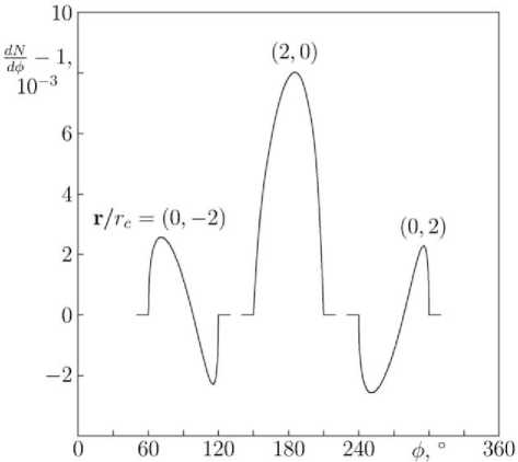
Figure 5 . Particle flux as a function of angle in the case of a moving magnetic cloud with a homogeneous magnetic field inside at r / r _c=(0, –2), (2, 0) (directly along the cloud path) and (0, 2). Cloud velocity v / c =2·10 ^–3 , parameters q =10 (particle energy ≈10 mc ² ), β=0.01 (gyroradius in the cloud field r g/ r c=0.1)

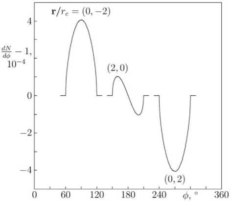
Figure 6 . The same for β=1 (gyroradius r _g/ r _c=10)

polar vectors for which the component normal to the plane changes sign). Thus, the reflection in the plane passing through an observer and the axis of cloud symmetry changes the sign of the magnetic field, thereby leading to a different physical situation and revealing itself in the asymmetric dependence of the flux on the angle. In the case of a hard magnetic mirror, this asymmetry is weak, whereas in the case of a weak field, on the contrary, the angular distribution is antisymmetric. Note that from angular distribution asymmetry we can determine such an important parameter as the magnetic field direction in a cloud.

The two adjacent regions with increased and decreased fluxes are observed by the URAGAN muon hodoscope. As an example in Figure 7, taken from [Yashin et al., 2015] , we present the result of recovery of the cosmic ray flux at the boundary of Earth’s magnetosphere as detected by the muon hodoscope from 08:00 to

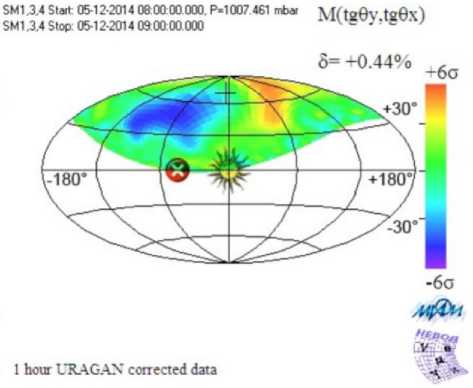
Figure 7 . Cosmic ray flux at the boundary of Earth’s magnetosphere as detected by the URAGAN muon hodoscope on May 12, 2014, averaged over the interval from 08:00 to 09:00 UT [Yashin et al., 2015] . The solar corona image in the center indicates the sunward direction, the cross on the left marks the direction of the interplanetary magnetic field line, the cross at the top is the direction of arrival of cosmic rays producing vertically incident muons. The parameter δ indicates the relative change in the total muon flux; the distribution by directions is given in units of statistical error

09:00 UT on December 5, 2014 Note that methods of processing URAGAN hodoscope data have been actively developing, which can automatically identify these regions of increased and decreased fluxes [Astapov et al., 2017; Getmanov et al., 2017a, b; Getmanov et al., 2019; Dobrovolsky et al., 2019] .

CONCLUSION

Let us briefly discuss advantages and disadvantages of our approach. The advantages include the ability to calculate directly observed anisotropy based on the simple assumption about isotropic nature of the particle flux incident from outside. In this case it turns out that the static magnetic field does not cause the anisotropy. Regions of varying (moving) magnetic field generate the anisotropy of the order of v / c ~10^–3 , where v is the solar wind velocity. Fast moving magnetic inhomogeneities make the largest contribution to the anisotropy.

The disadvantages indicate that the anisotropy is affected by not only the region of the heliosphere between the Sun and Earth, but also by the outer region if it has sufficiently strong magnetic inhomogeneities. The very assumption about incident flux isotropy is insufficiently justified either. There is no direct data on 10 GeV solar cosmic rays; and for the 500–1000 GeV cosmic rays it is known ([Berezinski et al., 1984] , P. 38) that their distribution is anisotropic, with anisotropy also being 10^–3. A similar anisotropy has been recently recorded in the PAMELA experiment for 1–20 TeV cosmic rays [Karelin et al., 2015] . Nevertheless, Formula (14) relating the flux at two points along one phase trajectory remains valid in general and can be applied to the analysis of data from a particle detector.

In the future, we plan to test the proposed approach, using a more realistic model of coronal mass ejection as an example.

This work was conducted in the framework of budgetary funding of the Geophysical Center of RAS, adopted by the Ministry of Science and Higher Education of the Russian Federation.